Difference: AmericanSteelTransshipmentProblem (2 vs. 3)
Revision 32008-02-16 - TWikiAdminUser
| Line: 1 to 1 | |||||||||||||||||||||||||||||||||||||||||||||||||||||||||||||||||||||||||||||||||||||||||
|---|---|---|---|---|---|---|---|---|---|---|---|---|---|---|---|---|---|---|---|---|---|---|---|---|---|---|---|---|---|---|---|---|---|---|---|---|---|---|---|---|---|---|---|---|---|---|---|---|---|---|---|---|---|---|---|---|---|---|---|---|---|---|---|---|---|---|---|---|---|---|---|---|---|---|---|---|---|---|---|---|---|---|---|---|---|---|---|---|---|
| |||||||||||||||||||||||||||||||||||||||||||||||||||||||||||||||||||||||||||||||||||||||||
| Deleted: | |||||||||||||||||||||||||||||||||||||||||||||||||||||||||||||||||||||||||||||||||||||||||
| < < |
<--
This topic can only be changed by:
| ||||||||||||||||||||||||||||||||||||||||||||||||||||||||||||||||||||||||||||||||||||||||
| Changed: | |||||||||||||||||||||||||||||||||||||||||||||||||||||||||||||||||||||||||||||||||||||||||
| < < | The American Steel Transshipment Problem | ||||||||||||||||||||||||||||||||||||||||||||||||||||||||||||||||||||||||||||||||||||||||
| > > | <-- This topic can only be changed by:
Case Study: The American Steel Transshipment Problem | ||||||||||||||||||||||||||||||||||||||||||||||||||||||||||||||||||||||||||||||||||||||||
Submitted: 15 Feb 2008 | |||||||||||||||||||||||||||||||||||||||||||||||||||||||||||||||||||||||||||||||||||||||||
| Changed: | |||||||||||||||||||||||||||||||||||||||||||||||||||||||||||||||||||||||||||||||||||||||||
| < < | Operations Research Areas: | ||||||||||||||||||||||||||||||||||||||||||||||||||||||||||||||||||||||||||||||||||||||||
| > > | Operations Research Topics: LinearProgramming, IntegerProgramming, NetworkOptimisation, TransshipmentProblem | ||||||||||||||||||||||||||||||||||||||||||||||||||||||||||||||||||||||||||||||||||||||||
Application Areas: Logistics | |||||||||||||||||||||||||||||||||||||||||||||||||||||||||||||||||||||||||||||||||||||||||
| Changed: | |||||||||||||||||||||||||||||||||||||||||||||||||||||||||||||||||||||||||||||||||||||||||
| < < | Problem Description | ||||||||||||||||||||||||||||||||||||||||||||||||||||||||||||||||||||||||||||||||||||||||
| > > | ContentsProblem Description | ||||||||||||||||||||||||||||||||||||||||||||||||||||||||||||||||||||||||||||||||||||||||
American Steel, an Ohio-based steel manufacturing company, produces steel at its two steel mills located at Youngstown and Pittsburgh. The company distributes finished steel to its retail customers through the distribution network of regional and field warehouses shown below:
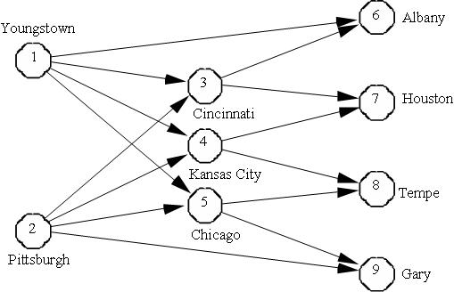 The network represents shipment of finished steel from American Steel's two steel mills located at Youngstown (node 1) and Pittsburgh (node 2) to their field warehouses at Albany, Houston, Tempe, and Gary (nodes 6, 7, 8 and 9) through three regional warehouses located at Cincinnati, Kansas City, and Chicago (nodes 3, 4 and 5). Also, some field warehouses can be directly supplied from the steel mills.
Table 1 presents the minimum and maximum flow amounts of steel that may be shipped between different cities along with the cost per 1000 ton/month of shipping the steel. For example, the shipment from Youngstown to Kansas City is contracted out to a railroad company with a minimal shipping clause of 1000 tons/month. However, the railroad cannot ship more than 5000 tons/month due the shortage of rail cars.
Table 1 Arc Costs and Limits
The network represents shipment of finished steel from American Steel's two steel mills located at Youngstown (node 1) and Pittsburgh (node 2) to their field warehouses at Albany, Houston, Tempe, and Gary (nodes 6, 7, 8 and 9) through three regional warehouses located at Cincinnati, Kansas City, and Chicago (nodes 3, 4 and 5). Also, some field warehouses can be directly supplied from the steel mills.
Table 1 presents the minimum and maximum flow amounts of steel that may be shipped between different cities along with the cost per 1000 ton/month of shipping the steel. For example, the shipment from Youngstown to Kansas City is contracted out to a railroad company with a minimal shipping clause of 1000 tons/month. However, the railroad cannot ship more than 5000 tons/month due the shortage of rail cars.
Table 1 Arc Costs and Limits
| |||||||||||||||||||||||||||||||||||||||||||||||||||||||||||||||||||||||||||||||||||||||||
| Changed: | |||||||||||||||||||||||||||||||||||||||||||||||||||||||||||||||||||||||||||||||||||||||||
| < < | Problem Formulation | ||||||||||||||||||||||||||||||||||||||||||||||||||||||||||||||||||||||||||||||||||||||||
| > > |
Return to top
Problem Formulation | ||||||||||||||||||||||||||||||||||||||||||||||||||||||||||||||||||||||||||||||||||||||||
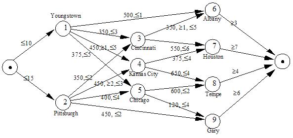
The American Steel Problem can be solved as a transshipment problem. The supply at the supply nodes is the maximum production at the steel mills, i.e., 10,000 and 15,000 for Youngstown and Pittsburgh respectively. The demand at demand nodes in given by the demand at the field warehouses and the other nodes are transshipment nodes. The costs and bounds on flow through the network are also given. The most compact formulation for this problem is a network formulation (see The Transshipment Problem for details).
| |||||||||||||||||||||||||||||||||||||||||||||||||||||||||||||||||||||||||||||||||||||||||
| Changed: | |||||||||||||||||||||||||||||||||||||||||||||||||||||||||||||||||||||||||||||||||||||||||
| < < | Computational Model | ||||||||||||||||||||||||||||||||||||||||||||||||||||||||||||||||||||||||||||||||||||||||
| > > |
Return to top
Computational Model | ||||||||||||||||||||||||||||||||||||||||||||||||||||||||||||||||||||||||||||||||||||||||
<--/twistyPlugin twikiMakeVisibleInline-->
We can use the AMPL model file transshipment.mod (see The Transshipment Problem in AMPL for details) to solve the American Steel Transshipment Problem. We need a data file to describe the nodes, arcs, costs and bounds. The node set is simply a list of the node names:
set NODES := Youngstown  Pittsburgh
             Cincinnati 'Kansas City' Chicago
             Albany      Houston      Tempe   Gary ;
Note that Kansas City must be enclosed in ' and ' because of the whitespace in the name.
The arc set is 2-dimensional and can be defined in a number of different ways:
# List of arcs
set ARCS := (Youngstown, Albany), (Youngstown, Cincinnati), ... , (Chicago, Gary) ;
# Table of arcs set ARCS: Cincinnati 'Kansas City' Chicago Albany Houston Tempe Gary := Youngstown + + + + - - - Pittsburgh + + + - - - + . . . # Array of arcs set ARCS := (Youngstown, *) Cincinnati 'Kansas City' Chicago Albany (Pittsburgh, *) Cincinnati 'Kansas City' Chicago Gary . . . (Chicago, *) Tempe Gary ;Since the node set is small and the arc set is "dense", i.e., many of the node pairs are represented in the arc set, we choose a table to define ARCS: set ARCS: Cincinnati 'Kansas City' Chicago Albany Houston Tempe Gary := Youngstown + + + + - - - Pittsburgh + + + - - - + Cincinnati - - - + + - - 'Kansas City' - - - - + + - Chicago - - - - - + + ;The NetDemand can be defined easily from the supply and demand. Since the default is 0 we don't need to define NetDemand for the transshipment nodes:
param      NetDemand :=
Youngstown -10000
Pittsburgh -15000
Albany       3000
Houston      7000
Tempe        4000
Gary         6000
 ;
We can use lists, tables or arrays to define the parameters for the American Steel Transhippment Problem, but in this case we will use a list and define multiple parameters at once. This allows us to "cut-and-paste" the parameters from the problem description. Note the use of . for parameters where the defaults will suffice (e.g., Lower for Youngstown and Albany):
param:                  	Cost    Lower  	Upper:=
Youngstown	Albany		500	.	1000
Youngstown	Cincinnati	350	.	3000
Youngstown	'Kansas City'	450	1000	5000
Youngstown	Chicago		375	.	5000
.
.
.
Chicago		Gary		120	.	4000
 ;
Note that the cost is in $/1000 ton, so we must divide the cost by 1000 in our script file before solving:
reset;

model transshipment.mod;

data steel.dat;

let {(m, n) in ARCS} Cost[m, n] := Cost[m, n] / 1000;

option solver cplex;
solve;

display Flow;
<--/twistyPlugin--> <--/twistyPlugin twikiMakeVisibleInline-->
We can define the PuLP/Dippy model using functions in transshipment_funcy.py
<--/twistyPlugin--> | |||||||||||||||||||||||||||||||||||||||||||||||||||||||||||||||||||||||||||||||||||||||||
| Changed: | |||||||||||||||||||||||||||||||||||||||||||||||||||||||||||||||||||||||||||||||||||||||||
| < < | Results | ||||||||||||||||||||||||||||||||||||||||||||||||||||||||||||||||||||||||||||||||||||||||
| > > |
Return to top
Results | ||||||||||||||||||||||||||||||||||||||||||||||||||||||||||||||||||||||||||||||||||||||||
Using transshipment.mod, and the data and script files defined in Computational Model we can solve the American Steel Transshipment Problem to get the optimal Flow variables:
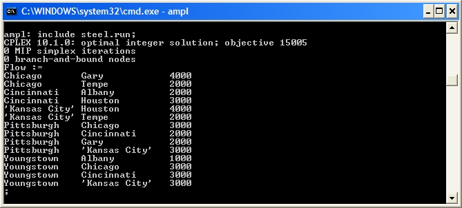 If the total supply is greater than the total demand, the transshipment problem will solve, but flow may be left in the network (in this case at the Pittsburgh node). In
 transshipment.mod we check that sum {n in NODES} NetDemand[n] <= 0 to ensure a problem is feasible before solving.
If total supply is less than demand (hence the problem is infeasible) we can add a dummy supply node (see with arcs to all the demand nodes. The optimal solution will show the "best" nodes to send the extra supply to.
| |||||||||||||||||||||||||||||||||||||||||||||||||||||||||||||||||||||||||||||||||||||||||
| Changed: | |||||||||||||||||||||||||||||||||||||||||||||||||||||||||||||||||||||||||||||||||||||||||
| < < | Conclusions | ||||||||||||||||||||||||||||||||||||||||||||||||||||||||||||||||||||||||||||||||||||||||
| > > |
Return to top
Conclusions | ||||||||||||||||||||||||||||||||||||||||||||||||||||||||||||||||||||||||||||||||||||||||
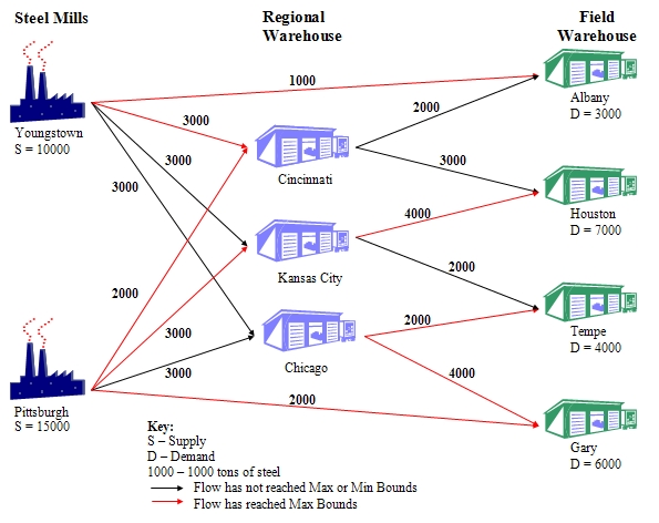
In order to minimise the monthly shipment costs, American Steel should follow the shipment plan shown in Table 3.
Table 3 Optimal Shipment Plan
| |||||||||||||||||||||||||||||||||||||||||||||||||||||||||||||||||||||||||||||||||||||||||
| Changed: | |||||||||||||||||||||||||||||||||||||||||||||||||||||||||||||||||||||||||||||||||||||||||
| < < | |||||||||||||||||||||||||||||||||||||||||||||||||||||||||||||||||||||||||||||||||||||||||
| > > | Return to top | ||||||||||||||||||||||||||||||||||||||||||||||||||||||||||||||||||||||||||||||||||||||||
| Changed: | |||||||||||||||||||||||||||||||||||||||||||||||||||||||||||||||||||||||||||||||||||||||||
| < < | Student Tasks | ||||||||||||||||||||||||||||||||||||||||||||||||||||||||||||||||||||||||||||||||||||||||
| > > |
Student Tasks | ||||||||||||||||||||||||||||||||||||||||||||||||||||||||||||||||||||||||||||||||||||||||
| |||||||||||||||||||||||||||||||||||||||||||||||||||||||||||||||||||||||||||||||||||||||||
| Added: | |||||||||||||||||||||||||||||||||||||||||||||||||||||||||||||||||||||||||||||||||||||||||
| > > | Return to top | ||||||||||||||||||||||||||||||||||||||||||||||||||||||||||||||||||||||||||||||||||||||||
| |||||||||||||||||||||||||||||||||||||||||||||||||||||||||||||||||||||||||||||||||||||||||
| Changed: | |||||||||||||||||||||||||||||||||||||||||||||||||||||||||||||||||||||||||||||||||||||||||
| < < |
| ||||||||||||||||||||||||||||||||||||||||||||||||||||||||||||||||||||||||||||||||||||||||
| > > |
| ||||||||||||||||||||||||||||||||||||||||||||||||||||||||||||||||||||||||||||||||||||||||
The network represents shipment of finished steel from American Steel’s two steel mills located at Youngstown (node 1) and Pittsburgh (node 2) to their field warehouses at Albany, Houston, Tempe, and Gary (nodes 6, 7, 8 and 9) through three regional warehouses located at Cincinnati, Kansas City, and Chicago (nodes 3, 4 and 5). Also, some field warehouses can be directly supplied from the steel mills.
The table below presents the minimum and maximum flow amounts of steel that may be shipped between different cities along with the cost per 1000 ton/month of shipping the steel. For example, the shipment from Youngstown to Kansas City is contracted out to a railroad company with a minimal shipping clause of 1000 tons/month. However, the railroad cannot ship more then 5000 tons/month due the shortage of rail cars.
Flow of goods (cases of beer in The Beer Distribution Problem, tons of steels here) through the network. In ???LINK??? A Transportation Problem all arcs from the supply nodes to the demand nodes existed (although in ???LINK??? Forestry Management we used upper bounds to removes some arcs). In The American Steel Problem, the network has transshipment nodes and arcs don't exist between all nodes. However, arcs must travel from one node to another. In AMPL we ???LINK??? declare the set of NODES and the set of ARCS between nodes:
# The set of all nodes in the network
set NODES;

# The set of arcs in the network
set ARCS within NODES cross NODES;
Now we define bounds on the flow (of our goods) along each arc:
# The minimum and maximum flow allowed along the arcs
param Min {ARCS} integer, default 0;
param Max {(m, n) in ARCS} integer, >= Min[m, n], default Infinity;
and finally declare our Flow variables:
# The flow of goods to be sent across an arc
var Flow {(m, n) in ARCS} >= Min[m, n], <= Max[m, n], integer;
2. FORMULATE THE OBJECTIVE FUNCTION
The objective of transshipment problems in general and The American Steel Problem in particular is to minimise the cost of shipping goods through the network:
# The cost of shipping 1 unit of goods (per time unit)
param Cost {ARCS};

# Minimise the total shipping cost
minimize TotalCost:
  sum {(m, n) in ARCS} Cost[m, n] * Flow[m, n];
3. FORMULATE THE CONSTRAINTS
All the nodes have supply and demand, demand = 0 for supply nodes, supply = 0 for demand nodes and supply = demand = 0 for transshipment nodes. Also, the supply and demand amounts must be integer to ensure a naturally integer solution (i.e., linear programming will provide an integer optimal solution).
# Each node has a (non-negative, integer) supply and a (non-negative, integer) demand
# Note. supply nodes have demand = 0 and vice versa,
# transshipment nodes have supply = demand = 0
param Supply {NODES} >= 0, integer, default 0;
param Demand {NODES} >= 0, integer, default 0;
The only constraints in the transshipment problem are flow conservation constraints. These constraints
simply state that the flow of goods into a node must be greater than the flow of goods out of a node.
# Must conserve flow in the network (goods cannot disappear!)
subject to ConserveFlow {n in NODES}:
  sum {m in NODES: (m, n) in ARCS} Flow[m, n] + Supply[n] =>
  sum {p in NODES: (n, p) in ARCS} Flow[n, p] + Demand[n];
For example, if a node has a supply of 10 units and has 10 units flowing in, then it can have no more than 20 units flowing out:
 Transshipment problems are often presented as a network formulation:
4. IDENTIFY THE DATA
The nodes of The American Steel Problem can be easily ???LINK??? defined using a list :
Transshipment problems are often presented as a network formulation:
4. IDENTIFY THE DATA
The nodes of The American Steel Problem can be easily ???LINK??? defined using a list :
set NODES := Youngstown  Pittsburgh
             Cincinnati 'Kansas City' Chicago
             Albany      Houston      Tempe   Gary ;
Note that Kansas City must be enclosed in ' and ' because of the whitespace in the name.
The arc set is 2-dimensional and can be ???LINK??? defined in a number of different ways :
# List of arcs
set ARCS := (Youngstown, Albany), (Youngstown, Cincinnati), ... , (Chicago, Gary) ;
# Table of arcs set ARCS: Cincinnati 'Kansas City' Chicago Albany Houston Tempe Gary := Youngstown + + + + - - - Pittsburgh + + + - - - + Cincinnati - - - + + - - 'Kansas City' - - - - + + - Chicago - - - - - + + ; # Array of arcs set ARCS := (Youngstown, *) Cincinnati 'Kansas City' Chicago Albany (Pittsburgh, *) Cincinnati 'Kansas City' Chicago Gary . . . (Chicago, *) Tempe Gary ;We can choose lists, tables or arrays to define the parameters for The American Steel Problem, but in this case we will use a list and ???LINK??? define multiple parameters at once. This allows us to "cut-and-paste" the parameters from the problem description. Note the use of . for parameters where the defaults will suffice (e.g., Min['Youngstown', 'Albany']):
param:                          Cost    Min     Max:=
Youngstown      Albany          500     .       1000
Youngstown      Cincinnati      350     .       3000
Youngstown     'Kansas City'    450     1000    5000
Youngstown      Chicago         375     .       5000
Pittsburgh      Cincinnati      350     .       2000
Pittsburgh     'Kansas City'    450     2000    3000
Pittsburgh      Chicago         400     .       4000
Pittsburgh      Gary            450     .       2000
Cincinnati      Albany          350     1000    5000
Cincinnati      Houston         550     .       6000
'Kansas City'   Houston         375     .       4000
'Kansas City'   Tempe           650     .       4000
Chicago         Tempe           600     .       2000
Chicago         Gary            120     .       4000
 ;
Note that the cost is in $/1000 ton, so we must divide the cost by 1000 before solving:
let {(m, n) in ARCS} Cost[m, n] := Cost[m, n] / 1000;
| | |||||||||||||||||||||||||||||||||||||||||||||||||||||||||||||||||||||||||||||||||||||||||


View topic | History: r24 < r23 < r22 < r21 | More topic actions...
Ideas, requests, problems regarding TWiki? Send feedback