Case Study: ATransshipmentProblem

Submitted: 15 Feb 2008

Operations Research Topics:

Application Areas: Logistics

Contents

• Problem Description
• Problem Formulation
• Computational Model
• Results
• Conclusions
• Extra for Experts
• StudentTasks

Problem Description

THE AMERICAN STEEL PROBLEM

American Steel, an Ohio-based steel manufacturing company, produces steel at its two steel mills located at Youngstown and Pittsburgh. The company distributes finished steel to its retail customers through the distribution network of regional and field warehouses shown below:

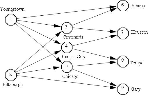
The network represents shipment of finished steel from American Steel’s two steel mills located at Youngstown (node 1) and Pittsburgh (node 2) to their field warehouses at Albany, Houston, Tempe, and Gary (nodes 6, 7, 8 and 9) through three regional warehouses located at Cincinnati, Kansas City, and Chicago (nodes 3, 4 and 5). Also, some field warehouses can be directly supplied from the steel mills.

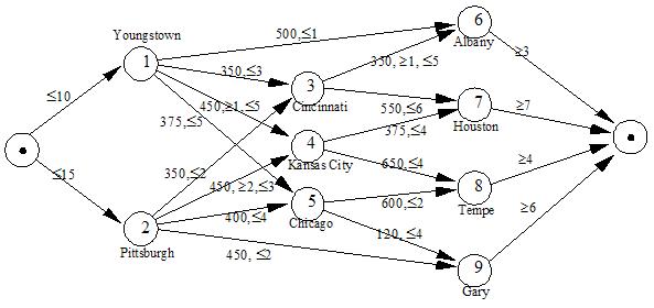
The table below presents the minimum and maximum flow amounts of steel that may be shipped between different cities along with the cost per 1000 ton/month of shipping the steel. For example, the shipment from Youngstown to Kansas City is contracted out to a railroad company with a minimal shipping clause of 1000 tons/month. However, the railroad cannot ship more then 5000 tons/month due the shortage of rail cars.

From node	To node	Cost	Minimum	Maximum
Youngstown	Albany	500	-	1000
Youngstown	Cincinnati	350	-	3000
Youngstown	Kansas City	450	1000	5000
Youngstown	Chicago	375	-	5000
Pittsburgh	Cincinnati	350	-	2000
Pittsburgh	Kansas City	450	2000	3000
Pittsburgh	Chicago	400	-	4000
Pittsburgh	Gary	450	-	2000
Cincinnati	Albany	350	1000	5000
Cincinnati	Houston	550	-	6000
Kansas City	Houston	375	-	4000
Kansas City	Tempe	650	-	4000
Chicago	Tempe	600	-	2000
Chicago	Gary	120	-	4000

The current monthly demand at American Steel’s four field warehouses is as follows:

Field Warehouses	Monthly Demand
Albany, N.Y.	3000
Houston	7000
Tempe	4000
Gary	6000

The Youngstown and Pittsburgh mills can produce up to 10,000 tons and 15,000 tons of steel per month, respectively. The management wants to know the least cost monthly shipment plan.

Return to top

Problem Formulation

1. IDENTIFY THE DECISION VARIABLES

The decision variables for this problem are the same as for the transportation problem, the Flow of goods (cases of beer in The Beer Distribution Problem, tons of steels here) through the network. In ???LINK??? A Transportation Problem all arcs from the supply nodes to the demand nodes existed (although in ???LINK??? Forestry Management we used upper bounds to removes some arcs). In The American Steel Problem, the network has transshipment nodes and arcs don't exist between all nodes. However, arcs must travel from one node to another. In AMPL we ???LINK??? declare the set of NODES and the set of ARCS between nodes:

# The set of all nodes in the network
set NODES;

# The set of arcs in the network
set ARCS within NODES cross NODES;

Now we define bounds on the flow (of our goods) along each arc:

# The minimum and maximum flow allowed along the arcs
param Min {ARCS} integer, default 0;
param Max {(m, n) in ARCS} integer, >= Min[m, n], default Infinity;

and finally declare our Flow variables:

# The flow of goods to be sent across an arc
var Flow {(m, n) in ARCS} >= Min[m, n], <= Max[m, n], integer;

2. FORMULATE THE OBJECTIVE FUNCTION

The objective of transshipment problems in general and The American Steel Problem in particular is to minimise the cost of shipping goods through the network:

# The cost of shipping 1 unit of goods (per time unit)
param Cost {ARCS};

# Minimise the total shipping cost
minimize TotalCost:
  sum {(m, n) in ARCS} Cost[m, n] * Flow[m, n];

3. FORMULATE THE CONSTRAINTS

All the nodes have supply and demand, demand = 0 for supply nodes, supply = 0 for demand nodes and supply = demand = 0 for transshipment nodes. Also, the supply and demand amounts must be integer to ensure a naturally integer solution (i.e., linear programming will provide an integer optimal solution).

# Each node has a (non-negative, integer) supply and a (non-negative, integer) demand
# Note. supply nodes have demand = 0 and vice versa,
# transshipment nodes have supply = demand = 0
param Supply {NODES} >= 0, integer, default 0;
param Demand {NODES} >= 0, integer, default 0;

The only constraints in the transshipment problem are flow conservation constraints. These constraints simply state that the flow of goods into a node must be greater than the flow of goods out of a node.

# Must conserve flow in the network (goods cannot disappear!)
subject to ConserveFlow {n in NODES}:
  sum {m in NODES: (m, n) in ARCS} Flow[m, n] + Supply[n] =>
  sum {p in NODES: (n, p) in ARCS} Flow[n, p] + Demand[n];

For example, if a node has a supply of 10 units and has 10 units flowing in, then it can have no more than 20 units flowing out:

Transshipment problems are often presented as a network formulation:

4. IDENTIFY THE DATA

The nodes of The American Steel Problem can be easily ???LINK??? defined using a list :

set NODES := Youngstown  Pittsburgh
             Cincinnati 'Kansas City' Chicago
             Albany      Houston      Tempe   Gary ;

Note that Kansas City must be enclosed in ' and ' because of the whitespace in the name.

The arc set is 2-dimensional and can be ???LINK??? defined in a number of different ways :

# List of arcs
set ARCS := (Youngstown, Albany), (Youngstown, Cincinnati), ... , (Chicago, Gary) ;

# Table of arcs
set ARCS:   Cincinnati 'Kansas City' Chicago Albany Houston Tempe Gary :=
Youngstown         +          +         +      +       -      -    -
Pittsburgh         +          +         +      -       -      -    +
Cincinnati         -          -         -      +       +      -    -
'Kansas City'      -          -         -      -       +      +    -
Chicago            -          -         -      -       -      +    + ;

# Array of arcs
set ARCS :=
(Youngstown, *)    Cincinnati 'Kansas City' Chicago Albany
(Pittsburgh, *)    Cincinnati 'Kansas City' Chicago Gary
.
.
.
(Chicago, *)       Tempe       Gary
 ;

We can choose lists, tables or arrays to define the parameters for The American Steel Problem, but in this case we will use a list and ???LINK??? define multiple parameters at once. This allows us to "cut-and-paste" the parameters from the problem description. Note the use of . for parameters where the defaults will suffice (e.g., Min['Youngstown', 'Albany']):

param:                          Cost    Min     Max:=
Youngstown      Albany          500     .       1000
Youngstown      Cincinnati      350     .       3000
Youngstown     'Kansas City'    450     1000    5000
Youngstown      Chicago         375     .       5000
Pittsburgh      Cincinnati      350     .       2000
Pittsburgh     'Kansas City'    450     2000    3000
Pittsburgh      Chicago         400     .       4000
Pittsburgh      Gary            450     .       2000
Cincinnati      Albany          350     1000    5000
Cincinnati      Houston         550     .       6000
'Kansas City'   Houston         375     .       4000
'Kansas City'   Tempe           650     .       4000
Chicago         Tempe           600     .       2000
Chicago         Gary            120     .       4000
 ;

Note that the cost is in $/1000 ton, so we must divide the cost by 1000 before solving:

let {(m, n) in ARCS} Cost[m, n] := Cost[m, n] / 1000;

Return to top

Computational Model

The computational model...

Return to top

Results

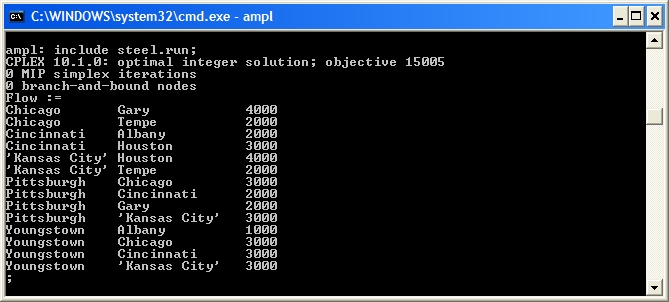
Implementing the usual script file with transshipment.mod and steel.dat (with the Cost modification) gives us the optimal Flow variables:

If the total supply is greater than the total demand, the transshipment problem will solve, but flow may be left in the network (in this case at the Pittsburgh node). If total supply is less than demand, then the problem becomes infeasible! Even in the case of infeasibility, it is preferable to solve the transshipment problem using a dummy supply node so that we can analyse where there is a shortfall in demand. We can balance the problem by either adding a dummy supply node with arcs to all the demand nodes or adding a dummy demand node with arcs from all the supply nodes: balance_transshipment.mod

# The following parameters are needed to use balance_transshipment.run
param difference;
param dummyDemandCost {NODES};
param dummySupplyCost {NODES};

balance_transshipment.run

let difference := (sum {s in NODES} Supply[s])
                - (sum {d in NODES} Demand[d]);
             
let NODES := NODES union {'Dummy'};             
if difference > 0 then
{
  print "Total Supply > Total Demand";
  print "Solving with dummy supply node...";
  let Demand['Dummy'] := difference;
  for {n in NODES : Supply[n] > 0} {
    let ARCS := ARCS union {(n, 'Dummy')};
    let Cost[n, 'Dummy'] := dummyDemandCost[n];
  }
}
else if difference < 0 then
{
  print "WARNING: Total Supply < Total Demand, problem is infeasible!";
  print "Solving with dummy demand node...";
  let Demand['Dummy'] := - difference;
  for {n in NODES : Demand[n] > 0} {
    let ARCS := ARCS union {('Dummy', n)};
    let Cost['Dummy', n] := dummySupplyCost[n];
  }
}; # else the problem is balanced

steel.run

# steel.run
#
# Written by Mike O'Sullivan & Cameron Walker 2004
#
# This file contains a script for sensitivity analysis
# of the American Steel transshipment model.
#
# Last modified: 27/2/2004

reset;

model transshipment.mod;
model balance_transshipment.mod;

data steel.dat;

let {(m, n) in ARCS} Cost[m, n] := Cost[m, n] / 1000;

for {n in NODES} {
  let dummyDemandCost[n] := 0;
  let dummySupplyCost[n] := 0;  
}

include balance_transshipment.run;

option solver cplex;

solve;

display Flow;  

Note We also add a ???LINK??? check statement to our model file to ensure the problem is balanced:

check : sum {n in NODES} Supply[n] = sum {n in NODES} Demand[n];

Our solution now shows that there is 5000 ton of steel remaining at the Pittsburgh Mill, i.e., the flow from Pittsburgh to Dummy is 5000.

POST-OPTIMAL ANALYSIS

Validation For our solution to be valid we need it to be integer. Observing the Flow values shows that it is in fact integer. Moreover, no branch-and-bound nodes were required to make it integer. The transshipment problem is also naturally integer (like the transportation problem), so solving it as a linear programme will give integer solutions. In fact, any network flow problem with integer supplies, demands and arc capacities has naturally integer solutions.

Parametric Analysis If ???LINK??? sensitivity analysis shows that improvements to the objective function may be achieved by changing problem data, then we may use ???LINK??? parametric analysis to see the effect of these changes.

.
.
.
include balance_transshipment.run;

option presolve 0;
option solver cplex;
option cplex_options 'presolve 0 sensitivity';
solve;

display Flow;

display _varname, _var.down, _var.current, _var.up, _var.rc;
display _conname, _con.down, _con.current, _con.up, _con.dual;

The sensitivity analysis shows that the solution is very sensitive to any changes in the constraint right-hand sides, with one exception ConserverFlow at Pittsburgh. However, we have variables on both sides of our constraints so we should expand our constraints to see what the right-hand side is:

For the supply nodes the right-hand side is the negative of the supply, for the demand nodes the right-hand side is the demand and for the transshipment nodes the right-hand side is 0. Thus, any changes we make to the supply or demand at the nodes will affect our optimal solution. The only exception is that the right-hand side of the ConserveFlow['Pittsburgh'] can decrease without affecting our solution. Since Pittsburgh is a supply node (so the right-hand side is the negative of the supply) this means we can increase the supply at Pittsburgh without affecting our solution. This makes sense as Pittsburgh already has excess supply.

However, it seems like we can improve our objective the most by decreasing the demand at Tempe (the shadow price is 1.125), but the Allowable Minimum is such that we cannot discern what the change will be (the solution will change immediately). We can see the effect by using an ???LINK??? AMPL loop :

.
.
.
display TotalCost;

set CHANGES;
param Objective {CHANGES};

param OldDemand;

let OldDemand := Demand['Tempe'];

let CHANGES := {100..1000 by 100}; 
for {i in CHANGES} {
  
  let Demand['Tempe'] := OldDemand - i;
  display Demand['Tempe'];

  # Rebalance the problem  
  include balance_transshipment.run;
  
  solve;
  
  let Objective[i] := TotalCost;
}

Note that we had to alter balance_transshipment.run to consider problems that have been balanced previously: balance_transshipment.run

let difference := (sum {s in NODES : s <> 'Dummy'} Supply[s])
                - (sum {d in NODES : d <> 'Dummy'} Demand[d]);
             
if 'Dummy' not in NODES then
  let NODES := NODES union {'Dummy'};
  
if difference > 0 then
{
  print "Total Supply > Total Demand";
  print "Solving with dummy supply node...";
  let Demand['Dummy'] := difference;
  for {n in NODES : Supply[n] > 0} {
    let ARCS := ARCS union {(n, 'Dummy')};
    let Cost[n, 'Dummy'] := dummyDemandCost[n];
  }
}
else if difference < 0 then
{
  print "WARNING: Total Supply < Total Demand, problem is infeasible!";
  print "Solving with dummy demand node...";
  let Demand['Dummy'] := - difference;
  for {n in NODES : Demand[n] > 0} {
    let ARCS := ARCS union {('Dummy', n)};
    let Cost['Dummy', n] := dummySupplyCost[n];
  }
}; # else the problem is balanced

The AMPL parametric analysis shows that, by decreasing the demand for steel at Tempe, we can get a consistent reduction in our objective function, even though this was not clear from our initial sensitivity analysis.

When we consider the sensitvity analysis for variable costs, we see that the only costs that affect our solution are the transportation costs from Pittsburgh and Youngstown to Chicago (all the other costs have Allowable Min and Allowable Max such that no "sensible" change would have any effect). Suppose American Steel are negotiating a new contract with the shipping company that takes their steel from Pittsburgh to Chicago. They estimate that they can get a reduction of around \$25/1000 ton of steel (taking the price from \$400/1000 ton to \$375/1000 ton), but want to know if they should negotiate for a lower price. The sensitivity analysis shows that below \$375/1000 ton the solution will change, so let's use parametric analysis to see what happens:

.
.
.
display TotalCost;

set CHANGES;
param Objective {CHANGES};

param OldCost;

let OldCost := Cost['Pittsburgh', 'Chicago'];

let CHANGES := {0..0.05 by 0.005}; 
for {i in CHANGES} {
  
  let Cost['Pittsburgh', 'Chicago'] := OldCost - i;
  display Cost['Pittsburgh', 'Chicago'];

  # Rebalance the problem  
  include balance_transshipment.run;
  
  solve;
  
  let Objective[i] := TotalCost;
}

The parametric analysis shows that the objective function decreases at a greater rate if the price drops below $375/1000 ton, so American Steel should try and negotiate the price down even further.

Return to top

Conclusions

There is quite a bit of information to summarise and many ways to present it. Some suggestions include:

1. Summarise the problem as usual and list the shipments that American Steel should make (similar to the transportation problem);
2. Summarise the problem as usual and present a table of shipments that American Steel should make;
3. Draw the network formulation for the problem (being sure to specify what the labels mean). Then draw the actual solution on top of the network formulation. You could colour code flows long arcs to show if they are at their bounds.

Implementation and Ongoing Monitoring

Given that the solution is very sensitive to the supply and demand amounts, careful consideration of the accuracy of these figures is important. Making sure that the bounds on the arcs are reliable is another concern.

Ongoing monitoring of the supply, demand and bounds will help American Steel to keep making good decisions. As shown in the parametric analysis, ongoing negotiation of transportation prices along important routes will help American Steel reduce their expenditure.

Return to top

Extra for Experts

Another common network flow problem that uses almost the same model as transshipment is the maximum flow problem. The objective of this problem is to maximise flow through the network. The only changes to transshipment.mod are:

1. A new variable FlowOut is introduced at each node;
2. FlowOut has lower and upper bounds, often the upper bound is set to as the Demand at the nodes;
3. FlowOut replaces Demand in the ConserveFlow constraints;
4. The ConserveFlow constraint becomes an equality constraint as all flow must be accounted for (no storage at the nodes);
5. Cost of transshipment is ignored;
6. The objective is to maximise the total flow out of the network sum {n in NODES} FlowOut[n];
7. The problem no longer needs to be balanced.

Maxflow.mod ???ATTACH MAXFLOW.MOD HERE???

If we set MaxOut to Demand for all nodes:

let {n in NODES} MaxOut[n] := Demand[n];

then we see that currently all the demands are being met via the American Steel distribution network (the total flow out = the total demand):

Return to top

Student Tasks

1. Solve The American Steel Problem. Write a management summary of your solution.

What to hand in Hand in your management summary.

EXTRA FOR EXPERTS' TASKS

1. American Steel are planning a marketing campaign to increase demand in their four markets Albany, Tempe, Houston and Gary. However, they would like to know the maximum demand their distribution network can handle (in each market) before they proceed. Write a script file that uses maxflow.mod and steel.dat to find the maximum demand they can supply in each market.

What to hand in Hand in your script file and a management summary of your solution.

Return to top