Case Study: The Cosmic Computers Problem
Submitted: 21 Sep 2012
Operations Research Topics: IntegerProgramming, FacilityLocationProblem
Application Areas: Industrial Planning
Contents
- Problem Description
- Problem Formulation
- Computational Model
- Results
- Conclusions
- Extra for Experts
- StudentTasks
Problem Description
The Cosmic Computer company wish to set up production in America. They are contemplating building production plants in up to 4 locations. Each location has planning restrictions that effectively determine the monthly production possible in each location. The monthly fixed costs of the different locations have been calculated by the accounting department, and are listed below:| Location | Monthly Fixed Cost |
|---|---|
| San Francisco | $70,000 |
| Los Angeles | $70,000 |
| Phoenix | $65,000 |
| Denver | $70,000 |
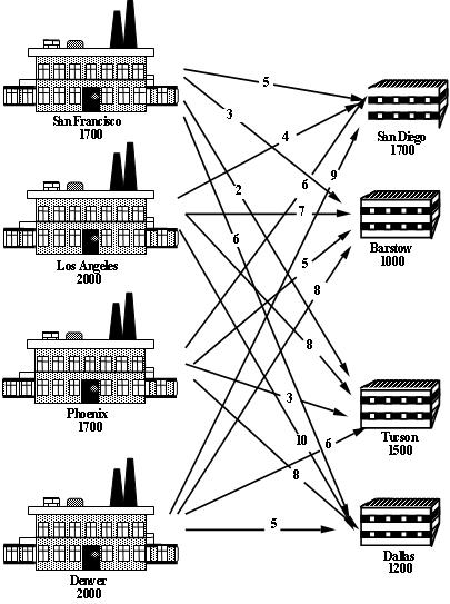 Where should the company set up their plants to minimise their total costs (fixed plus transportation)?
Like most businesses, Cosmic Computers are big Excel users, but don't know much about optimisation. They would like to develop an AMPL model that uses SolverStudio to allow them to solve this problem using Excel.
Return to top
Where should the company set up their plants to minimise their total costs (fixed plus transportation)?
Like most businesses, Cosmic Computers are big Excel users, but don't know much about optimisation. They would like to develop an AMPL model that uses SolverStudio to allow them to solve this problem using Excel.
Return to top
Problem Formulation
This problem is a facility location problem where the master-slave constraints control the existence of supply nodes for a transportation problem. Traditional transportation problem formulations are as follows:![\[ \begin{array}{r@{\,}r@{\,}l} \min & \displaystyle \sum_{i \in {\cal S}} \sum_{j \in {\cal D}} c_{ij} & x_{ij} \\ \text{subject to} & \displaystyle \sum_{j \in {\cal D}} & x_{ij} = s_i, i \in {\cal S} \\ & \displaystyle \sum_{i \in {\cal S}} & x_{ij} = d_j, j \in {\cal D} \end{array} \]](/pub/OpsRes/CosmicComputersSolverStudio/latex26453b5d201d586f3f1b8c1e74613609.png)
The decisions are two-fold: 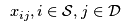 determine where to ship the computers, so we need to add binary variables that govern which of the supply nodes exist, i.e.,
  that are 1 if
  exists and 0 otherwise.
2. Formulate the Objective Function
exists and 0 otherwise.
2. Formulate the Objective Function
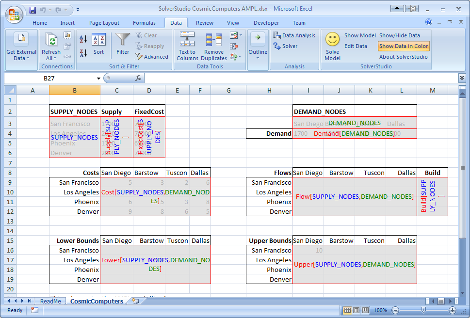
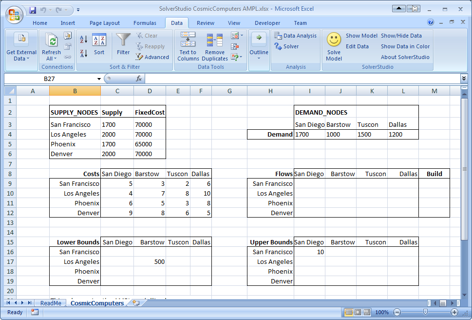 We need to define (i.e. give names to) these 'data items' on the spreadsheet, as shown below. These names must match those given in the AMPL model for the parameters and decision variables. The parameter data items include the supplies (cells B2:B6), demands (cells I4:L4), the flow costs, and the bounds. The decision variables are the flows and build decisions. One possible way of defining these data items is shown below. Notice, for example, that the Supply (C3:C6) and FixedCosts (D3:D6) are indexed over the SUPPLY_NODES (B3:B6) given in first column of the same table. The Demand is similarly defined over DEMAND_NODES listed in the first row of the Demand table. The Cost (C9:F12) is similarly defined, but note now that that indices are not the rows and column titles for the table, but actually refer to the SUPPLY_NODES and DEMAND_NODES defined not in the cost table, but in the supply and demand tables.
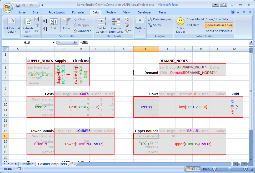
 Another way of defining these items, in which we always index over the rows and columns of the actual table defining the data, is shown below. Either of these approaches works fine.
 The spreadsheet file SolverStudioCosmicComputersAMPL-Incomplete.xlsx only has some of the data items defined. We will add the missing data items, and then solve this model.
If you have not yet installed SolverStudio, then either please visit SolverStudio to download this software, or, in the Engineering Science labs, install it from the path FoE Shared drive (S:) : ENGSCI : ug-courses : Courses : EngSci355.
Download and Open the Example Spreadsheet
1/ Download and save the spreadsheet file SolverStudioCosmicComputersAMPL-Incomplete.xlsx to the hard disk.
2/ Open your downloaded spreadsheet.
3/ Switch to the Data tab in Excel, and use SolverStudio's "Show/Hide Data" and "Show Data in Color" buttons to see the current data items.
Add the Missing Data Items
4/ Click SolverStudio's "Edit Data" button to open SolverStudio's Data Items editor.
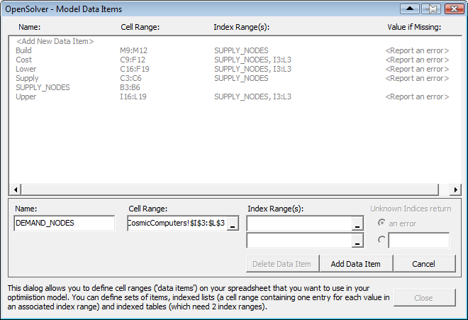
5/ We wish to define DEMAND_NODES. Make sure that the "Add New Data Item" item is selected. Then, type in a 'Name' of DEMAND_NODES, click the 'Cell Range' box, and then drag over the Demand cells (I3:L3). (Excel may add dollars and the sheet name; that's ok.) This data item is an AMPL set, and so we leave the 'Index Range(s)' blank. Click 'Add Data Item'.
The spreadsheet file SolverStudioCosmicComputersAMPL-Incomplete.xlsx only has some of the data items defined. We will add the missing data items, and then solve this model.
If you have not yet installed SolverStudio, then either please visit SolverStudio to download this software, or, in the Engineering Science labs, install it from the path FoE Shared drive (S:) : ENGSCI : ug-courses : Courses : EngSci355.
Download and Open the Example Spreadsheet
1/ Download and save the spreadsheet file SolverStudioCosmicComputersAMPL-Incomplete.xlsx to the hard disk.
2/ Open your downloaded spreadsheet.
3/ Switch to the Data tab in Excel, and use SolverStudio's "Show/Hide Data" and "Show Data in Color" buttons to see the current data items.
Add the Missing Data Items
4/ Click SolverStudio's "Edit Data" button to open SolverStudio's Data Items editor.
5/ We wish to define DEMAND_NODES. Make sure that the "Add New Data Item" item is selected. Then, type in a 'Name' of DEMAND_NODES, click the 'Cell Range' box, and then drag over the Demand cells (I3:L3). (Excel may add dollars and the sheet name; that's ok.) This data item is an AMPL set, and so we leave the 'Index Range(s)' blank. Click 'Add Data Item'.
 6/ Repeat the previous step to add the 'Demand' data item (cell range I4:L4), which is indexed over DEMAND_NODES. To create this index, click on the first (i.e. top) "Index Range(s)" entry box, and either type in the name of an already defined data item (DEMAND_NODES), or type in or drag over the appropriate cells (I3:L3 in this case). Then click 'Add Data Item'.
7/ Repeat the previous step to add the 'FixedCost' data item (cell range D3:D6), which is indexed over SUPPLY_NODES (or B3:B6 if you prefer).
8/ Create the 'Flow' data item (which has SUPPLY_NODES (B3:B6) as its first index, and DEMAND_NODES (I4:L4) as its second, or cells H9:H12 and I8:L8 if you prefer).
9/ Still staying in the Data Items editor, check each data item is correct by clicking on it in the data items list, and observing the cells SolverStudio highlights. Correct any mistakes you have made.
10/ Close the Data Items editor.
Check and Solve using AMPL
11/ If you cannot see the AMPL model text, click SolverStudio's 'Show Model' button to view the SolverStudio model editor. Note that you can print this model using SolverStudio's File... Print menu. (This menu also lets you print the model output.)
12/ By carefully working through the AMPL model, check that you have now defined as data items all the parameters in the AMPL model that have data on the spreadsheet, and all the decision variables in the AMPL model that need to be written to the spreadsheet.
13/ Use SolverStudio's Language menu to check that AMPL is selected as the language.
14/ We now wish to solve this problem using AMPL. If you have downloaded SolverStudio yourself, then you will need to install the AMPL Student Version; the SolverStudio AMPL menu has a command to do this automatically. This will take a minute or two.
15/ Use the SolverStudio 'Solve Model' button (or File... Solve, which has the shortcut key F5) to run and solve this model, and check that the flows and build decisions appear on the spreadsheet.
16/ SolverStudio creates a data file from your spreadsheet data. You can view this using the AMPL menu item 'View Last Data File'. This can be helpful in debugging.
17/ Save your spreadsheet to keep the changes you have made.
18/ SolverStudio provides access to various sources of online AMPL documentation under the AMPL menu. Try opening one of these.
Congratulations; you now have a working AMPL model running in SolverStudio, and have completed this SolverStudio tutorial.
Return to top
6/ Repeat the previous step to add the 'Demand' data item (cell range I4:L4), which is indexed over DEMAND_NODES. To create this index, click on the first (i.e. top) "Index Range(s)" entry box, and either type in the name of an already defined data item (DEMAND_NODES), or type in or drag over the appropriate cells (I3:L3 in this case). Then click 'Add Data Item'.
7/ Repeat the previous step to add the 'FixedCost' data item (cell range D3:D6), which is indexed over SUPPLY_NODES (or B3:B6 if you prefer).
8/ Create the 'Flow' data item (which has SUPPLY_NODES (B3:B6) as its first index, and DEMAND_NODES (I4:L4) as its second, or cells H9:H12 and I8:L8 if you prefer).
9/ Still staying in the Data Items editor, check each data item is correct by clicking on it in the data items list, and observing the cells SolverStudio highlights. Correct any mistakes you have made.
10/ Close the Data Items editor.
Check and Solve using AMPL
11/ If you cannot see the AMPL model text, click SolverStudio's 'Show Model' button to view the SolverStudio model editor. Note that you can print this model using SolverStudio's File... Print menu. (This menu also lets you print the model output.)
12/ By carefully working through the AMPL model, check that you have now defined as data items all the parameters in the AMPL model that have data on the spreadsheet, and all the decision variables in the AMPL model that need to be written to the spreadsheet.
13/ Use SolverStudio's Language menu to check that AMPL is selected as the language.
14/ We now wish to solve this problem using AMPL. If you have downloaded SolverStudio yourself, then you will need to install the AMPL Student Version; the SolverStudio AMPL menu has a command to do this automatically. This will take a minute or two.
15/ Use the SolverStudio 'Solve Model' button (or File... Solve, which has the shortcut key F5) to run and solve this model, and check that the flows and build decisions appear on the spreadsheet.
16/ SolverStudio creates a data file from your spreadsheet data. You can view this using the AMPL menu item 'View Last Data File'. This can be helpful in debugging.
17/ Save your spreadsheet to keep the changes you have made.
18/ SolverStudio provides access to various sources of online AMPL documentation under the AMPL menu. Try opening one of these.
Congratulations; you now have a working AMPL model running in SolverStudio, and have completed this SolverStudio tutorial.
Return to top
 . (Note that you can also use SolverStudio's AMPL menu to access the AMPL documentation.)
 This shows that
  Now the LP relaxation
  Here the optimal integer solution is found at the second node and then the rest of the tree (6 branch-and-bound nodes in all) is used to ensure this is the optimum. CPLEX is very careful with its selection of a branching variable. Here, it branches on
  Notice that the branch-and-bound tree is larger (8 nodes as opposed to 6), so this selection strategy did not work as well as the CPLEX default.
While solving the Cosmic Computers Problem we have explored many of the "behind the scenes" work that CPLEX does for you. See Integer Programming with AMPL for more examples. In the Extra for Experts we will see another technique called constraint branching.
Return to top
Notice that the branch-and-bound tree is larger (8 nodes as opposed to 6), so this selection strategy did not work as well as the CPLEX default.
While solving the Cosmic Computers Problem we have explored many of the "behind the scenes" work that CPLEX does for you. See Integer Programming with AMPL for more examples. In the Extra for Experts we will see another technique called constraint branching.
Return to top
 Return to top
 The sum of the three non-zero
  3 or
3 or  2. First, let's branch up:
 Our solution is integer so we can fathom this node. Now let's drop the Up constraint and branch down:
 This solution still has fractional
  Return to top
- Where to build the plants?
- Where to ship the computers?
determine where to ship the computers, so we need to add binary variables that govern which of the supply nodes exist, i.e., that are 1 if exists and 0 otherwise.
2. Formulate the Objective Function
The cost of transporting good through the network is already incorporated into the transportation problem objective, now we have to add the fixed (construction + maintenance) cost  :
:
![\[ \min \sum_{i \in {\cal S}} \sum_{j \in {\cal D}} c_{ij} x_{ij} + \sum_{i \in {\cal S}} C_i z_i \]](/pub/OpsRes/CosmicComputersSolverStudio/latex3eb875a228804876749e5dd54b0280ea.png)
3. Formulate the Constraints
:
The constraints are the same as the transportation problem formulation, except that the supply is determined by the construction (or not) of a plant:
![\[ \sum_{j \in {\cal D}} x_{ij} = s_i z_i, i \in {\cal S} \]](/pub/OpsRes/CosmicComputersSolverStudio/latex2d6a08916c2f1d6d313a5c0c8c0c2ed4.png) and we need to (at least) meet demand, but the formulation no longer needs to be balanced (otherwise we would always build all our construction plants):
and we need to (at least) meet demand, but the formulation no longer needs to be balanced (otherwise we would always build all our construction plants):
![\[ \sum_{i \in {\cal S}} x_{ij} \geq d_j, j \in {\cal D} \]](/pub/OpsRes/CosmicComputersSolverStudio/latex0946f5c33c1780d39232c3cffc2dab5b.png)
4. Identify the data
The data in this problem is the same as that required for a transportation problem, i.e.,  ,
,  ,
,  , etc except that the fixed costs also needs to be specified.
Return to top
, , , etc except that the fixed costs also needs to be specified.
Computational Model
Since a transportation problem is embedded within the Cosmic Computers Problem, we will start with the AMPL model filetransportation.mod (see The Transportation Problem in AMPL for details):
set SUPPLY_NODES;
set DEMAND_NODES;

param Supply {SUPPLY_NODES} >= 0, integer;
param Demand {DEMAND_NODES} >= 0, integer;

param Cost {SUPPLY_NODES, DEMAND_NODES} default 0;

param Lower {SUPPLY_NODES, DEMAND_NODES}
  integer default 0;
param Upper {SUPPLY_NODES, DEMAND_NODES}
  integer default Infinity;

var Flow {i in SUPPLY_NODES, j in DEMAND_NODES}
  >= Lower[i, j], <= Upper[i, j], integer;

minimize TotalCost:
  sum {i in SUPPLY_NODES, j in DEMAND_NODES}
    Cost[i, j] * Flow[i, j];

subject to UseSupply {i in SUPPLY_NODES}:
  sum {j in DEMAND_NODES} Flow[i, j] = Supply[i];

subject to MeetDemand {j in DEMAND_NODES}:
  sum {i in SUPPLY_NODES} Flow[i, j] = Demand[j];
We add new decision variables that decide if we build the production plants or not:
var Build {SUPPLY_NODES} binary;
We define a new parameter for the fixed cost (of construction + maintenance):
param FixedCost {SUPPLY_NODES};
We incorporate the fixed cost into the objective function and the Build variables into the supply constraints and change the supply constraints since the problem may not be balanced:
minimize TotalCost:
  sum {i in SUPPLY_NODES, j in DEMAND_NODES}
    Cost[i, j] * Flow[i, j] +
  sum {i in SUPPLY_NODES} FixedCost[i] * Build[i];

subject to UseSupply {i in SUPPLY_NODES}:
  sum {j in DEMAND_NODES} Flow[i, j] <= Supply[i] * Build[i];
SolverStudio does not use a .run file, and so we simply add our data, solve and output commands below the model.
data SheetData.dat; # Get data from the spreadsheet

check : sum {s in SUPPLY_NODES} Supply[s] >= sum {d in DEMAND_NODES} Demand[d];

option solver cplex; # Use this for the student version of AMPL
solve;

option display_1col 9999999; # a magic line SolverStudio needs
display Build > Sheet;
display Flow > Sheet;
Note that we have included a check command to ensure there is enough supply.
The spreadsheet file with this model (but still with some more work to do, as we discuss next) is SolverStudioCosmicComputersAMPL-Incomplete.xlsx.
For this problem, our data includes supplies and demands, lower and upper bounds on the flows, and costs. Note that only some routes have lower and upper bounds; a blank entry in one of these tables means AMPL uses the default values (0 and infinity) given in the model.
We need to define (i.e. give names to) these 'data items' on the spreadsheet, as shown below. These names must match those given in the AMPL model for the parameters and decision variables. The parameter data items include the supplies (cells B2:B6), demands (cells I4:L4), the flow costs, and the bounds. The decision variables are the flows and build decisions. One possible way of defining these data items is shown below. Notice, for example, that the Supply (C3:C6) and FixedCosts (D3:D6) are indexed over the SUPPLY_NODES (B3:B6) given in first column of the same table. The Demand is similarly defined over DEMAND_NODES listed in the first row of the Demand table. The Cost (C9:F12) is similarly defined, but note now that that indices are not the rows and column titles for the table, but actually refer to the SUPPLY_NODES and DEMAND_NODES defined not in the cost table, but in the supply and demand tables.
Another way of defining these items, in which we always index over the rows and columns of the actual table defining the data, is shown below. Either of these approaches works fine.
The spreadsheet file SolverStudioCosmicComputersAMPL-Incomplete.xlsx only has some of the data items defined. We will add the missing data items, and then solve this model.
If you have not yet installed SolverStudio, then either please visit SolverStudio to download this software, or, in the Engineering Science labs, install it from the path FoE Shared drive (S:) : ENGSCI : ug-courses : Courses : EngSci355.
Download and Open the Example Spreadsheet
1/ Download and save the spreadsheet file SolverStudioCosmicComputersAMPL-Incomplete.xlsx to the hard disk.
2/ Open your downloaded spreadsheet.
3/ Switch to the Data tab in Excel, and use SolverStudio's "Show/Hide Data" and "Show Data in Color" buttons to see the current data items.
Add the Missing Data Items
4/ Click SolverStudio's "Edit Data" button to open SolverStudio's Data Items editor.
5/ We wish to define DEMAND_NODES. Make sure that the "Add New Data Item" item is selected. Then, type in a 'Name' of DEMAND_NODES, click the 'Cell Range' box, and then drag over the Demand cells (I3:L3). (Excel may add dollars and the sheet name; that's ok.) This data item is an AMPL set, and so we leave the 'Index Range(s)' blank. Click 'Add Data Item'.
6/ Repeat the previous step to add the 'Demand' data item (cell range I4:L4), which is indexed over DEMAND_NODES. To create this index, click on the first (i.e. top) "Index Range(s)" entry box, and either type in the name of an already defined data item (DEMAND_NODES), or type in or drag over the appropriate cells (I3:L3 in this case). Then click 'Add Data Item'.
7/ Repeat the previous step to add the 'FixedCost' data item (cell range D3:D6), which is indexed over SUPPLY_NODES (or B3:B6 if you prefer).
8/ Create the 'Flow' data item (which has SUPPLY_NODES (B3:B6) as its first index, and DEMAND_NODES (I4:L4) as its second, or cells H9:H12 and I8:L8 if you prefer).
9/ Still staying in the Data Items editor, check each data item is correct by clicking on it in the data items list, and observing the cells SolverStudio highlights. Correct any mistakes you have made.
10/ Close the Data Items editor.
Check and Solve using AMPL
11/ If you cannot see the AMPL model text, click SolverStudio's 'Show Model' button to view the SolverStudio model editor. Note that you can print this model using SolverStudio's File... Print menu. (This menu also lets you print the model output.)
12/ By carefully working through the AMPL model, check that you have now defined as data items all the parameters in the AMPL model that have data on the spreadsheet, and all the decision variables in the AMPL model that need to be written to the spreadsheet.
13/ Use SolverStudio's Language menu to check that AMPL is selected as the language.
14/ We now wish to solve this problem using AMPL. If you have downloaded SolverStudio yourself, then you will need to install the AMPL Student Version; the SolverStudio AMPL menu has a command to do this automatically. This will take a minute or two.
15/ Use the SolverStudio 'Solve Model' button (or File... Solve, which has the shortcut key F5) to run and solve this model, and check that the flows and build decisions appear on the spreadsheet.
16/ SolverStudio creates a data file from your spreadsheet data. You can view this using the AMPL menu item 'View Last Data File'. This can be helpful in debugging.
17/ Save your spreadsheet to keep the changes you have made.
18/ SolverStudio provides access to various sources of online AMPL documentation under the AMPL menu. Try opening one of these.
Congratulations; you now have a working AMPL model running in SolverStudio, and have completed this SolverStudio tutorial.
Return to top
Results
The output shows that CPLEX has not required any branch-and-bound nodes again. Is this problem also naturally integer? We can check by solving the LP relaxation usingoption relax_integrality 1 in our AMPL model.
Unfortunately, our problem is not naturally integer. CPLEX performs a lot of "clever tricks" to solve mixed-integer programmes quickly. Let's look at the effect of some of these techniques.
First, we can see what is happening in the branch-and-bound tree by setting the CPLEX options for displaying the branch-and-bound process: mipdisplay 2 gives a moderate amount of information about the process and mipinterval 1 displays this information for every node. For detailed information on setting CPLEX options in AMPL see ILOG's AMPL CPLEX User Guide
This shows that Node 0 (the LP relaxation) is solved, then an integer solution is found quickly with 6 cuts. There are many methods at work here, including: - A relaxation induced neighbourhood search (RINS) heuristic;
- A repair heuristic that tries to from integer solutions from fractional ones;
- Application of cuts to the LP relaxation;
- Careful selection of variables to branch on.
rinsheur -1 and repairtries -1) and see what happens (Note To see the true effect of these changes you will have to make changes to your script file, restart AMPL and run your script again. Otherwise, AMPL will use your old solution and the effect of your changes will not be obvious):
Now the LP relaxation Node 0 is solved, but then cuts are generated (indicated by Node 0+) and after 2 cuts are added an integer solution is found, shown by *. After 9 cuts are generated another integer solution is found (hence another *) and this is the optimal solution. Cuts are linear constraints that are added to the LP relaxation to remove fractional solutions. There is a vast amount of literature on cuts for integer programming (try "integer programming cut" on Google), but we will not delve into it here. Let's turn off all the cuts (CPLEX option mipcuts -1) and see what happens:
Here the optimal integer solution is found at the second node and then the rest of the tree (6 branch-and-bound nodes in all) is used to ensure this is the optimum. CPLEX is very careful with its selection of a branching variable. Here, it branches on Build['Denver'] even though this variable is integer in the LP relaxation. Instead of using the default CPLEX selection rules for the branching variable, let's branch on the fractional variable that is closest to integer (CPLEX option varselect -1):
Notice that the branch-and-bound tree is larger (8 nodes as opposed to 6), so this selection strategy did not work as well as the CPLEX default.
While solving the Cosmic Computers Problem we have explored many of the "behind the scenes" work that CPLEX does for you. See Integer Programming with AMPL for more examples. In the Extra for Experts we will see another technique called constraint branching.
Return to top
Conclusions
As with the Brewery Problem, the solution to the Cosmic Computers Problem can be presented in many ways. Figure 1 gives a graphical solution to the Cosmic Computers Problem. Figure 1 Solution to the Cosmic Computers Problem
Return to top
Extra for Experts
Another form of branch and bound implements branches on constraints that should take integer values. For example, in the Cosmic Computers Problem the sum of any subset ofBuild variables should be integer. Consider the LP relaxation solution:
The sum of the three non-zero Build variables is 2.82 (2 dp), but it should be integer. We can remove the fractional part by forcing this sum to be either 3 or 2. First, let's branch up:
Our solution is integer so we can fathom this node. Now let's drop the Up constraint and branch down:
This solution still has fractional Build variables. We can add further constraint branches to continue searching from this node:
Return to top
Student Tasks
- Solve the Cosmic Computers Problem. Write a management summary of your solution. What to hand in Your management summary.
- Experts Only Complete the branch-and-bound process using constraint branches on fractional sums of the
Buildvariables. Draw your branch-and-bound tree as shown above (in the Extra for Experts section). Be sure to indicate what branches you used. Briefly (1 paragraph) compare your experience with constraint branching to the variable branching used in CPLEX. What to hand in Hand in your drawing of your branch-and-bound tree along with your conclusions about the effectiveness of constraint branching compared with variable branching.


| I | Attachment | History | Action | Size | Date | Who | Comment |
|---|---|---|---|---|---|---|---|
| |
SolverStudioCosmicComputersAMPL-Incomplete.xlsx | r2 r1 | manage | 20.5 K | 2012-09-24 - 23:21 | AndrewMason | CosmicComputers Spreadsheet model with data items still to be finished |
Topic revision: r5 - 2019-08-12 - TWikiAdminUser

Ideas, requests, problems regarding TWiki? Send feedback