The Transportation Problem

Introduction

The transportation problem is one of the simplest forms of network optimisation.

The network is bi-partite, i.e., it can be split into two sets of nodes with all arcs going from one set to the other. One set ${\cal S}$ is called the supply nodes and the other set ${\cal D}$ is called the demand nodes. The arcs ${\cal A}$ are all arcs directed from a supply node to a demand node, i.e., ${\cal A} = {\cal S} \times {\cal D}$ . Any supply of goods to the network arrives at the supply nodes, denote this $s_i, i \in {\cal S}$ , and any demand for goods is realised at the demand nodes where it leaves the network, denote this $d_j, j \in {\cal D}$ . 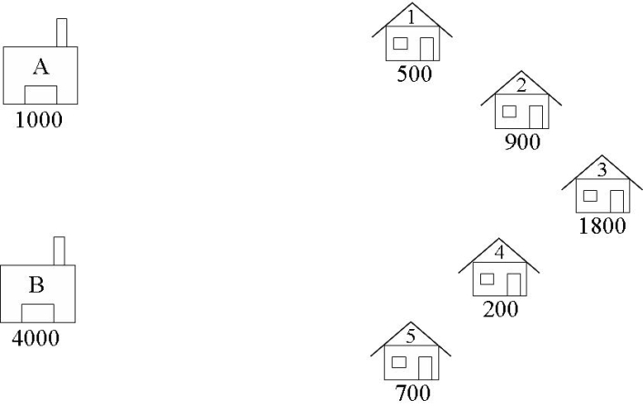Figure 1 shows the supply and demand nodes for the Brewery Problem with node labels and the supply and demand at the nodes given. Thus 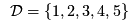${\cal S} = \{ A, B \}$ , ${\cal D} = \{ 1, 2, 3, 4, 5 \}$ , , , , , etc.

Figure 1 The nodes for the Brewery Problem

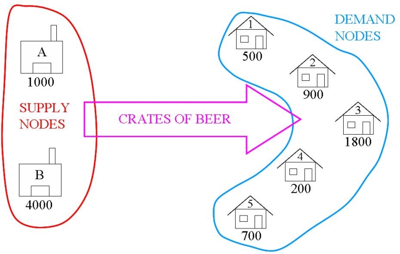
The arcs in the Brewery Problem carry crates of beer from the supply nodes (warehouses) to the demand nodes (bars) as shown in Figure 2. In this problem there are no restrictions of the arcs, so ${\cal A} = \{ (A, 1), (A, 2), (A, 3), (A, 4), (A, 5), (B, 1), (B, 2), (B, 3), (B, 4), (B, 5) \}$ .

Figure 2 The arcs carry crates of beer from the supply nodes to the demand nodes

In the transportation problem there is a cost $c_{ij}(x)$ associated with carrying goods from the supply node $i \in {\cal S}$ to the demand node $j \in {\cal D}$ along arc . In the classical transportation problem this is a unit cost per item, i.e., $c_{ij}(x) = c_{ij} x$

In a transportation problem we need to decide what quantity of goods to deliver along each arc to minimise the total transportation cost of delivering goods.

Formulating the Transportation Problem

Transportation problem are network optimisation problems. Network optimisation problems are solved using mathematical programming. Thus, to formulate a transportation problem we use the 4 steps for formulating a mathematical programme:

Identify the Decision Variables
Formulate the Objective Function
Formulate the Constraints
Identify the Data

Identify the Decision Variables

The decision variables in the transportation problem are the quantity of goods to carry along each arc, i.e., $x_{ij}, (i, j) \in {\cal A}$ . Note that $(i, j) \in {\cal A}$ means that $i \in {\cal S}$ and $j \in {\cal D}$ . Usually, these variables are integer and nonegative, i.e., $x_{ij} \in \mathbb{Z}_+$ .

Formulate the Objective Function

The objective in the transportation problem is to minimise the total transportation cost along the arcs, i.e.,

$\min \sum_{i \in {\cal S}} \sum_{j \in {\cal D}} c_{ij} x_{ij}$

Formulate the Constraints

The constraints in the transportation are simple: 1) use all the supply of goods; 2) meet all the demand of goods. These may be expressed concisely:

$\begin{align*} \sum_{j \in {\cal D}} x_{ij} &= s_i, i \in {\cal S} \\ \sum_{i \in {\cal S}} x_{ij} &= d_j, j \in {\cal D} \end{align*}$

Identify the Data

The data for the transportation problem is also straightforward to determine. We need to identify the supply nodes ${\cal S}$ and the demand nodes ${\cal D}$ , the supply and demand amounts, i.e., $s_i, i \in {\cal S}$ , $d_j, j \in {\cal D}$ , and the cost of transportation $c_{ij}$ from each supply node $i \in {\cal S}$ to each demand node $j \in {\cal D}$ .

Unbalanced Transportation Problems

The transportation problem we consider here must be balanced, i.e., $\sum_{i \in {\cal S}} s_i = \sum_{j \in {\cal D}} d_j$ , for the problem to be feasible. If a problem is not balanced then either there is an excess supply or an excess demand. These two factors can be incorporated by adjusting the relational operators on the constraints, e.g., for over supply change the supply constraint to

$\sum_{j \in {\cal D}} x_{ij} \leq s_i, i \in {\cal S}$

However, if the problem data changes, then the formulation may need to change. An easier way to deal with unbalanced transportation is to add dummy nodes to either the supply nodes (in the case of excess demand) or the demand nodes (in the case of excess supply). The supply (respectively demand) for the dummy node is simply the excess amount of demand (supply, respectively). There could also be a cost associated with goods coming from a dummy supply node, e.g., a penalty cost for buying in extra goods, or goods going to a dummy demand node, e.g., a salvage cost for unwanted items.

Restricting the Arcs

The arcs between the supply nodes and demand nodes may be restricted in two ways:

there may be bounds on the amount of goods that an arc may carry;
some arcs may not exist, i.e., there is no way to transport goods from a particular supply node to a particular demand node.

Dealing with bounds is done by adding bounds to the decision variables, i.e.,

$l_{ij} \leq x_{ij} \leq u_{ij}, (i, j) \in {\cal A}$

Dealing with non-existent arcs is more complicated. One way is to price the arc out of the solution, i.e., add a big cost (often referred to as a big- cost), so the arc will not be used. Sometimes it is not easy to determine a cost that is big enough to remove the arc from the final solution, but not so big that it distorts the solution process. The easiest way is to introduce bounds with default values, e.g., 0 for the lower bounds and $\infty$ for the upper bounds, and then set the upper bound of the banned arcs to be 0. This way no goods will be delivered along this arc.

Naturally Integer Solutions

The transportation problem is often an integer programme as the quantity of good delivered along the arcs must be integer. However, if the supply, demand and variable bounds are integer, then the transportation problem will have naturally integer solutions. This means that any solution found using linear programming will have integer values. This is a property that is common to other network optimisation problems, e.g., the transshipment problem.

Solving the Transportation Problem with OR Software

Using AMPL/CPLEX

To see examples of transportation problems, check out some of the transportation problem case studies:

Results from OpsRes web retrieved at 01:08 (GMT)

BreweryProblem

r10 - 2008-04-02 - 11:30 MichaelOSullivan

\usepackage{amsmath} Case Study: Submitted: Operations Research Topics: Application Areas: Contents Problem Description Problem Description Return...

ForestryProblem

r9 - 2008-04-03 - 01:38 MichaelOSullivan

\usepackage{amsmath} Case Study: Submitted: Operations Research Topics: Application Areas: Contents Problem Description Problem Description Return...

Number of topics: 2

-- MichaelOSullivan - 02 Apr 2008

Topic revision: r13 - 2019-11-11 - MichaelOSullivan