Case Study: Modelling Requests to a Courier Service
Submitted: 9 Aug 2009
Application Areas: Logistics
Contents
Problem Description
A courier company offers two services: an Inner City delivery service that delivers packages within the Inner City area in under an hour; a Metropolitan delivery service that delivers packages within the Metropolitan area in less than 4 hours.
An Inner City courier leaves the distribution centre if EITHER there are 10 deliveries to make OR it has been 15 minutes since the "oldest" delivery request arrived, i.e., the first request that arrived after the last delivery run departed. A Metropolitan courier leaves the distribution centre if EITHER there are 30 deliveries to make OR it has been 30 mins since the oldest delivery arrived. The courier company works for 8 hours a day and starts each day with no deliveries to make.
The courier company has collected data on the time between requests for both Inner City and Metropolitan deliveries as well as the time to make Inner City and Metropolitan deliveries. They want to know how many deliveries their Inner City and Metropolitan couriers make each day and also how long they are on the road during a day.
Return to top
Problem Formulation
To simplify the modelling we will
abstract 4 sections of the problem:
- Requests for Inner City deliveries;
- Requests for Metropolitan deliveries;
- Delivery runs for Inner City deliveries;
- Delivery runs for Metropolitan deliveries.
We start by assuming we can model these accurately using random variables, so we can concentrate on the remaining logic in the system.
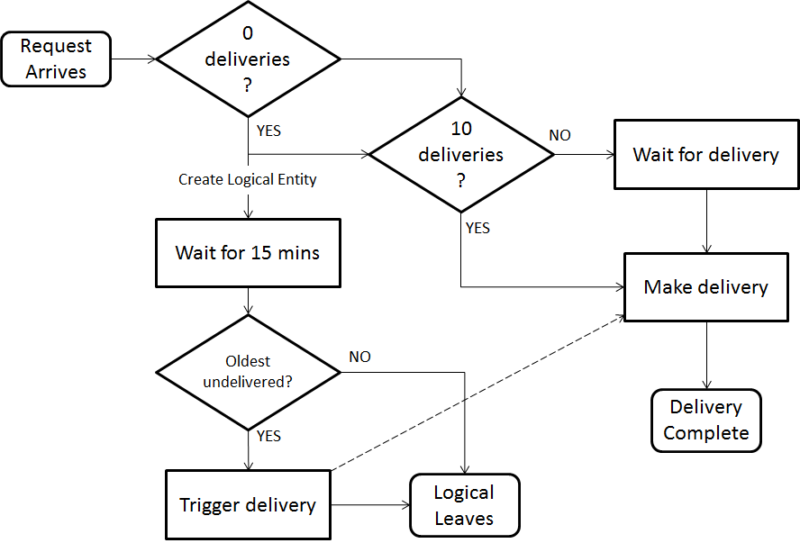
Figure 1 shows a flow diagram for the Inner City deliveries (note that a flowchart for the Metropolitan deliveries would be similar).
Figure 1 Flow Diagram for Inner City Deliveries
The way to implement this flow digram will differ depending on the simulation modelling tools used.
Return to top
Computational Model
To model the flow digram from
Figure 1 we first abstract the delivery requests and request runs as Arena submodels. The submodel for requests only generates requests, so a single submodel with only an exit point is needed. The submodel for a delivery run has the load of deliveries as input and outputs the load of deliveries after the delivery run finishes, so it has a single entry and exit point. The following
flash tutorial shows how to add the appropriate submodels in Arena:
Adding submodels for Courier Model
Table 1 Submodel Inputs
| Name |
Requests for Inner City Delivery |
| Number of Entry Points |
0 |
| Number of Exit Points |
1 |
| Name |
Requests for Metropolitan Delivery |
| Number of Entry Points |
0 |
| Number of Exit Points |
1 |
| Name |
Inner City Delivery Run |
| Number of Entry Points |
1 |
| Number of Exit Points |
1 |
| Name |
Metropolitan Delivery Run |
| Number of Entry Points |
1 |
| Number of Exit Points |
1 |
Table 1 shows the input value for the submodels.
Next, we want queues that store delivery entities until a delivery run occurs. We
define a boolean variable Loading Inner City that is 1 when an inner city courier may be loaded for delivery and 0 otherwise. We then
add a Hold module that stores deliveries until
Loading Inner City is 1. Remember that
Hold modules that
Scan for Condition only scan for the condition when a calendar event occurs. The next
flash tutorial shows how to
add a Hold module and
a Variable to implement this queue for Inner City deliveries.
Table 2 also summarises the input for the
Variable and
Hold modules.
Adding waiting queue for Courier Model
Table 2 Inputs for the
Variable and
Hold modules
| Name |
LoadingInnerCity |
| Initial Values |
0 |
| Name |
Wait for Inner City Delivery |
| Type |
Scan for Condition |
| Condition |
LoadingInnerCity == 1 |
Next, we want to create logical entities to take care of triggering delivery runs if the oldest delivery request has waited long enough. First, we
create an Expression that acts like a constant and stores the maximum time a delivery will wait before a courier run must deliver it.
Table 3 shows the input for this
Expression.
Table 3 Expression Input
| Name |
InnerCityMaxTime |
| Expression Values |
15 |
Note that the main difference between
Variables and
Expressions is that
Variables can change during a simulation. The value of an
Expression may change, but the actual
Expression will not. Note also that we could have simply "hard coded" the 15 into our model, but by using
Expressions we can easily change this time later if the courier operation changes.
Now, we
add a Variable that holds the time the oldest undelivered inner city delivery request arrived.
Table 4 shows the input for this
Variable.
Table 4 Variable Input
| Name |
InnerCityOldestArrival |
Each time a delivery request comes in we
use a Decide module to check if there are any other requests waiting. If there are no other deliveries waiting we note down its arrival time in
InnerCityOldestArrival using an Assign module and
create a timing entity using a Separate module. The duplicate entity then waits for the maximum time before a delivery run must deliver the oldest request (i.e.,
InnerCityMaxTime)
using a Delay module and then leaves the system. This may seem like a waste of simulation modules, but the departure of this duplicate entity from the model creates a calendar event which will cause all
Hold modules using
Scan for Condition to check their conditions. The original request joins the queue of requests waiting to be delivered (it will be the first one in the queue of course). The following
flash tutorial shows how to create the timing entity for the Inner City deliveries:
Adding timing entity to Courier Model
Table 5 Module inputs
| Name |
Any Inner City Deliveries Waiting? |
| Type |
2-way by Condition |
| If |
Expression |
| Value |
NQ(Wait for Inner City Delivery.Queue) > 0 |
| Name |
Set Inner City Oldest Arrival |
| Assignments (secondary dialog via Add button) |
| |
Type |
Variable |
| |
Variable Name |
InnerCityOldestArrival |
| |
New Value |
TNOW |
| Name |
Create Inner City Timer |
| Type |
Duplicate Original |
| # of Duplicates |
1 |
| Name |
Wait Inner City Max Time |
| Delay Time |
InnerCityMaxTime |
| Units |
Minutes |
| Name |
Dispose Inner City Timer |
Table 5 shows the inputs for the modules added.
Next, we create logical entities to trigger a delivery if:
- The amount of time since the oldest delivery arrived has reached the maximum time;
- The number of deliveries waiting has reached the maximum load.
The arrival of a new delivery creates a calendar event, as does the disposal of the timing entity created just before.
Hold modules will scan the simulation state each calendar event, so we can use one of these to trigger a delivery if either the maximum number of requests have been received or the maximum time for a request to wait has expired. Once a delivery run is needed, we simply "free" the requests being stored by setting the
LoadingInnerCity boolean variable to 1 (i.e., true). We then hold the logical entity until the deliveries have been loaded before returning it to the first
Hold module to wait for the next required delivery run. Note the use of a
Create module to create a single logical entity at the start of the simulation.
Table 6 shows the inputs to the 4 modules added.
Adding trigger entity to Courier Model
Table 6 Inputs for trigger modules
| Name |
Create Inner City Logical Entity |
| Entity Type |
InnerCityLogical |
| Max Arrivals |
1 |
| First Creation |
0.0 |
| Name |
Wait for Inner City Trigger |
| Type |
Scan for Condition |
| Condition |
( NQ(Wait for Inner City Delivery.Queue) >= InnerCityMaxLoad ) || ( TNOW - InnerCityOldestArrival >= InnerCityMaxTime ) |
| Name |
Start Inner City Loading |
| Assignments (secondary dialog via Add button) |
| |
Type |
Variable |
| |
Variable Name |
LoadingInnerCity |
| |
New Value |
1 |
| Name |
Wait for Inner City Loading |
| Type |
Scan for Condition |
| Condition |
NQ(Wait for Inner City Delivery.Queue) == 0 |
Now that we can trigger the loading of a delivery run, we want to combine all the deliveries into a single load, finish loading and make a delivery run. Once the run is finished we want to separate the deliveries and let them leave the system. First, we create a variable
NumberInnerCityLoad to record the number of requests in the load. This is set at the same time loading starts, in the
Start Inner City Loading Assign module. Next, we send requests from
Wait for Inner City Delivery to a
Batch module to be joined into a load. The size of the load for this particular delivery is recorded in an
Assign module and the loading is finished (i.e.,
LoadingInnerCity is set to 0 - false). Then the load is delivered and split into the original requests (using a
Separate module) to keep the count of requests in and out of the system accurate.
Table 7 shows the inputs to the modules extended/added.
Adding deliveries to Courier Model
Table 7 Inputs for delivery modules
| Name |
Start Inner City Loading |
| Assignments (secondary dialog via Add button) |
| |
Type |
Variable |
| |
Variable Name |
NumberInnerCityLoad |
| |
New Value |
NQ(Wait for Inner City Delivery.Queue) |
| Name |
Load Inner City Deliveries |
| Batch Size |
NumberInnerCityLoad |
| Name |
Inner City Delivery Loaded |
| Assignments (secondary dialog via Add button) |
| |
Type |
Attribute |
| |
Variable Name |
NumInLoad |
| |
New Value |
NumberInnerCityLoad |
| |
Type |
Variable |
| |
Variable Name |
LoadingInnerCity |
| |
New Value |
0 |
| Name |
Inner City Delivery Finished |
| Type |
Split Existing Batch |
| Name |
Dispose Inner City Delivery |
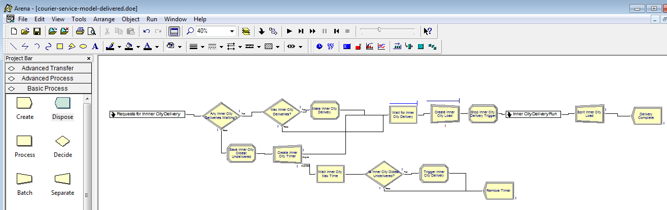
Now the logic of the Inner City part of the model is complete except for the arrivals and delivery runs. You complete Inner City model should look like that in
Figure 2.
Figure 2 Courier Model with complete Inner City logic
Next you will have to repeat the previous steps to build the Metropolitan part of the model. You can cut-and-paste modules in the flowchart view, but you will need to be careful to rename everything correctly.
Initial Distributions
Once you have completed both the Inner City and Metrpolitan parts of the model, you will need to add some distributions to "drive" your simulation. To start off with we will try some simple distributions. Use exponential interarrival times with mean 10 minutes and 20 minutes for Inner City and Metropolitan delivery requests (make sure to use EXPO(10) and EXPO(20) for the first arrival times too). We will use triangular distributions with min, mode and max of 10, 15, 20 and 25, 45, 90 for Inner CIty and Metropolitan delivery runs respectively. If you are unsure how to add and edit
Create and
Process modules, you should complete the
Output Buffering case study before continuing. Add the appropriate
Create and
Process modules to your
submodels. Connect them to the appropriate entry

and exit

points. Make sure you create different entities for each type of delivery and different resources for each type of delivery run. Finally, make sure you have an infinite number of couriers by editing the capacity of your Resources (click on the
Resources module in the
Basic Process template and look for
Capacity..
Now run your model for 50 replications. Each replication should run for 8 hours (i.e., 1 day of the courier operation) and the Base Time Units are minutes.
Debugging
You should notice that your model appears to "stall". If you look carefully you will see the logic entity that triggers Inner City delivery runs in an infinite loop. This happens because our hold condition is not quite correct. We rely on a request arriving and resetting the oldest delivery time. However, this does not happen before the truck is loaded, so the initial trigger hold does not work. We need to wait for a delivery after we load the truck. By adding an extra condition to the timing trigger, we can fix the problem.
Figure 3 shows this extra condition, that the delivery queue must have at least one delivery AND that the oldest delivery has been there for too long for a delivery run to take place.
Figure 3 Extra condition for timing trigger
 Figure 4
 Initial output from the Courier Model

After debugging and re-running you model you should get the output shown in
Figure 4, such as 0.5881 Inner City couriers being used on average and 18.84 Inner City delivery runs on average. However, we are just using some very crude estimates of input data to verify our model.
You can also use animation to check your model, such as animating queues and times to make sure the maximum load and maximum time restrictions are enforced. You can visualise the utilisation of the couriers and the number of each type of courier on the road at any one time:
Adding animation to Courier Model
Finding Input Distributions
As discussed previously, the courier company has recorded data on their delivery requests and delivery runs. This data is given
courier.xls.
We can use Arena's built-in Input Analyzer to determine distributions that fit the data well. First, we need to break the data up into separate text files as shown in
Figure 5.
Figure 5 Splitting data into text files

Then, we can use the Input Analyzer:
Analysing Inner City delivery requests
The Input Analyzer uses the
Chi Square and
Kolmogorov-Smirnov goodness-of-fit tests to determine which distributions fit best.
Once you have determined the best distributions, you can cut-and-paste their expressions into the appropriate submodels and run your simulation model again. Some results are shown in
Figure 6.
Figure 6 Results after input analysis

Using the Data
IMPORTANT You should save your model file under a new name before adding the empirical distributions as shown below. In the
Results section we will compare the 2 model files.
Instead of using the Input Analyzer to estimate distributions, we can use the
empirical distribution. The empirical distribution uses the histogram of the data to create a cumulative distribution function which it then uses to generate either discrete or continuous observations. In this example we will use the continuous distribution to generate interarrival times and processing times, i.e., the time taken for a courier run.
Determining the Empirical Distribution
Once you have changed the generation of delivery requests and the time taken to do courier runs to use empirical distributions, you can run your model again. However, you may get ant error complaining about using a value of 0.00 for an interarrival time. The first entry of your empirical distrubutions is (0.00, 0.00, ...), i.e., there is a very small (0.00 to 3 significant figures) chance of an observation of 0.00. If this happens an infinite number of times for an interarrival time (very small probability, but theoretically possible), then there may be an infinite loop, so Arena does not allow this. Simply remove the first 2 0.00 entries (thus removin the possibility of a 0.00 interarrival time, a reasonable assumption) and your Arena model will run.
Return to top
Results
Now we have finished building simulation models with different input distributions, we will compare our models. We can compare two simulations by creating data files giving output for each replication and comparing them in Arena's Output Analyzer.
First, add a Statistic to both models that records the average utilization of the Inner City Courier and the Metropolitan Courier.
Adding Output Statistics to Courier Model
Repeat this for your simulation model that uses the fitted distributions, but
make sure to give your output files different names. Next, we can use the Output Analyzer to compare the different models.
Comparing Courier Models
Figure 7 shows the confidence intervals generated by Output Analyzer. They measure the difference of the mean values, i.e., average number of busy couriers, for the inner city couriers and the metropolitan couriers. The difference is the mean from the fitted distribution model (input) minus the mean from the empirical distribution model (empirical). Notice that both confidence intervals span 0, so there is no evidence of any difference between the means. We can reduce the size of the confidence intervals by reducing the variance, i.e., running more replications.
Figure 7 Results after input analysis
 Return to top
Conclusions
The simulation model of the courier company provides different measurements of several aspects of the courier service. In this case study we looked mainly at the average number of couriers needed for both inner city and metropolitan deliveries.
We considered this statistic when using a couple of different models, one that estimated distributions for the data and one that use the empirical distribution of the data, i.e., it modelled the data explicitly.
The simulation results showed that there was no evidence to reject the hypothesis that both distributions gave the same mean, i.e., average number of couriers busy, for both the inner city and metropolitan couriers. This means that we could use either approach and our results would be statistically equivalent.
Return to top
Extra for Experts
Arena enables you to be more selective about how random numbers are used in your simulations. This may allow you to get more accuracy in your estimates with less replications. It can also allow you to improve accuracy when comparing simulations.
First, you need to add a
SEEDS element to your model. Then, you add the seed to your random number expressions. The following flash movie shows how to do this and also uses the
SEEDS element so that common random numbers are used across replications. Be sure to save a copy of your model before making changes.
Using a SEEDS element
Figure 8 shows the results for courier usage when using the empirical distribution and random numbers as usual, common random numbers and antithetic random numbers.
Figure 8 Courier Usage (Empirical Distribution) with different random number utilisation

- Using random numbers as usual

- Using common random numbers

- Using antithetic random numbers
In this case the common random numbers improved the estimate, but the antithetic random numbers did not.
Using the same random numbers in the same way in two models reduces the variance when comparing models. Comparing the courier model with fitted distributions to the model with the empirical distribution when both models are using random numbers in the same way, even without
Common or
Antithetic, gives a comparison with less variance.
Figure 9 shows the Output Analyzer results for the previous models (without the
SEEDS element - the first and third confidence intervals) and the new models (with the
SEEDS element without
Common or
Antithetic turned on - the second and last intervals).
Figure 9 Output Analyzer Results
 Return to top


