Case Study: The Brewery Logistics Problem

Submitted: 2 Apr 2008

Operations Research Topics: LinearProgramming, IntegerProgramming, NetworkOptimisation, TransportationProblem

Application Areas: Logistics

Problem Description

A boutique brewery has two warehouses from which it distributes beer to five carefully chosen bars. At the start of every week, each bar sends an order to the brewery's head office for so many crates of beer, which is then dispatched from the appropriate warehouse to the bar. The brewery would like to have an interactive computer program which they can run week by week to tell them which warehouse should supply which bar so as to minimize the costs of the whole operation.

For example, suppose that at the start of a given week the brewery has 1000 cases at warehouse A, and 4000 cases at warehouse B, and that the bars require 500, 900, 1800, 200, and 700 cases respectively.

The transportation costs are given in Table 1.

Table 1 Transportation costs from warehouses to bars

Cost ($/crate)	Warehouse A	Warehouse B
Bar 1	2	3
Bar 2	4	1
Bar 3	5	3
Bar 4	2	2
Bar 5	1	3

Which warehouse should supply which bar?

Return to top

Problem Formulation

Since crates of beer are being shipped from the warehouses to the bars, this problem is a bipartite network and can be modelled as a transportation problem.

The supply nodes are the warehouses, the demand nodes are the bars. The total supply is 1,000 + 4,000 = 5,000 and the total demand is 500 + 900 + 1,800 + 200 + 700 = 4,100, so the problem is unbalanced. We can either alter the balanced formulation to incorporate this or add a dummy demand node to receive the extra supply.

Return to top

Computational Model

Since this is a transportation problem we can use the AMPL model file for transportation problems.

The data file will have the supply nodes as the warehouses:

set SUPPLY_NODES := A B ;

and the demand nodes as the bars:

set DEMAND_NODES := 1 2 3 4 5 ;

The supply and demand is given and can be specified:

param Supply :=
A          1000
B          4000
 ;

param Demand :=
1            500
2            900
3          1800
4            200
5            700
 ;

Finally, the transportation costs are easier to specify using a transposed table:

param Cost (tr) :
     A    B :=
1    2    3
2    4    1
3    5    3
4    2    2
5    1    3
 ;

Note that since the problem is not balanced, the AMPL script file transportation.run (see Transportation Problems in AMPL for details) automatically adds a dummy demand node to the problem.

The AMPL model file transportation.mod also ensures the supply, demand and bound variables are integer so that only linear programming will be necessary (as we will get naturally integer solutions, see The Transportation Problem for details).

Return to top

Results

By inserting

data brewery.dat;

into transportation.run (see Transportation Problems in AMPL for details) we can solve the Brewery Problem. Figure 1 shows the AMPL output with the solution.

Figure 1 AMPL output for the Brewery Problem

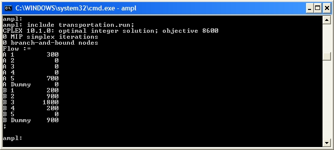This shows that the optimal solution is to make the shipments shown in Table 1.

* Table 1* Optimal shipments for the Brewery Problem

Shipment (crates)	Warehouse A	Warehouse B
Bar 1	300	200
Bar 2	-	900
Bar 3	-	1800
Bar 4	-	200
Bar 5	700	-

There are 900 crates left at Warehouse B.

Notice that CPLEX did not need to use any branch-and-bound nodes, i.e., no integer programming was required. This confirms that a transportation problem has naturally integer solutions. By specifying the supply, demand and bound parameters be integer we guarantee that only linear programming needs to be used.

Sensitivity Analysis

??? Up to here ??? Once you have solved The Beer Distribution Problem, you may want to check to see if there are any "easy" changes you could make to improve the objective. An initial way of looking for these changes is by performing sensitivity analysis on the problem data.

\begin{verbatim} # brewery.run reset;

model transportation.mod; data brewery.dat;

option solver cplex;

option presolve 0; # Turn off the AMPL presolve option cplex_options 'presolve 0 sensitivity'; # Turn off the CPLEX presolve, # Turn on the sensitivity analysis solve;

display Flow;

display _varname, _var, _var.rc, _var.current, _var.up, _var.down; display _conname, _con.body, _con.slack, _con.dual, _con.current, _con.up, _con.down; \end{verbatim}

The sensitivity analysis shows that the current solution is largely unaffected by changes in the transportation costs. The two exceptions are the transportation costs from Warehouse A to Bar 1 and from Warehouse B to Bar 1. The transportation cost from Warehouse A to Bar 1 can only increase from 2 to 3 before a solution change will occur. Similarly, the cost of transportation from Warehouse B to Bar 1 can only decrease from 3 to 2 before causing a solution change .

The sensitivity analysis also shows that a change in any of the constraints will cause the solution to change, except for the supply at Warehouse B. This supply can decrease to 3100 before any change in the solution happens. However, changing the supply at Warehouse B will not change the objective function value as {\tt EnoughSupply['B']} has a dual value (i.e., shadow price) of 0.

Return to top

Conclusions

There are many ways to present the solution to The Beer Distribution Problem: as a list of shipments, in a table, etc. You can use AMPL's {\tt display}, {\tt print} and {\tt printf} commands to create formatted output that can be easily used in your management summary. The following file was produced by an AMPL script file (the actual numbers have been removed):

brewery.out

\begin{verbatim} TRANSPORTATION SOLUTION -- Non-zero shipments TotalCost = __

Ship _ crates of beer from warehouse A to pub 1 Ship _ crates of beer from warehouse A to pub 5 Ship _ crates of beer from warehouse B to pub 1 Ship _ crates of beer from warehouse B to pub 2 Ship __ crates of beer from warehouse B to pub 3 Ship _ crates of beer from warehouse B to pub 4 \end{verbatim}

This information gives rise to the following management summary:

The Beer Distribution Problem

Mike O'Sullivan, 1234567

We are minimising the transportation cost for a brewery operation. The brewery transports cases of beer from its warehouses to several bars.

The brewery has two warehouses (A and B respectively) and 5 bars (1, 2, 3, 4 and 5).

The supply of crates of beer at the warehouses is:

______

The forecasted demand (in crates of beer) at the bars is:

______

The cost of transporting 1 crate of beer from a warehouse to a bar is given in the following table:

______

To minimise the transportation cost the brewery should make the following shipments:

The total transportation cost of this shipping schedule is $_____.

Analysis of Data Parameters

The current solution is robust under changes to all the costs except for the following transportation costs:

______ to _____ which can only ______ to _____; and,

__________ to _____ which can only ______ to _____.

However, any change in the amount of supply at the warehouses or the demand at the bars will cause the solution to change with the following exception:

The ______ at ______ can ______ to ______ .

If this ______ occurs then the objective function value ______ by ______ per unit ______ .

Implementation and Ongoing Monitoring

As always, the first step towards Implementation is a good management summary. In this case, the sensitivity analysis shows that the solution is very sensitive to the supply and demand amounts. Since the demand is forecasted, any implementation of the solution would be very dependent on excellent demand forecasting.

Ongoing Monitoring may take the form of:

Updating your data files and resolving as the data changes (changing costs, supplies, demands);
Resolving our model for new nodes (e.g., new warehouses or bars);
Looking to see if cheaper transportation options are available along routes where the transportation cost affects the optimal solution (e.g., how much total savings can we get by reducing the transportation cost from Warehouse B to Bar 1).

Return to top

Extra for Experts

You can use AMPL as a scripting language to generalise your models. For example, you can solve The Beer Distribution Problem for differing supplies and demands using the {\tt balanced_transportation.mod} model file, an extra model file {\tt balance.mod} and a script file {\tt balance.run}. The {\tt balance.mod} file declares three new parameters:

\begin{verbatim} # The following parameters are needed to use balance.run param difference; # The difference between total supply and total demand

param dummyDemandCost {SUPPLY_NODES}; # The cost of sending supply to a dummy demand node param dummySupplyCost {DEMAND_NODES}; # The cost of getting supply from a dummy supply node \end{verbatim}

and the {\tt balance.run} file automatically balances the data:

\begin{verbatim} let difference := (sum {s in SUPPLY_NODES} Supply[s]) - (sum {d in DEMAND_NODES} Demand[d]);

if difference > 0 then { let DEMAND_NODES := DEMAND_NODES union {'Dummy'}; let Demand['Dummy'] := difference; let {s in SUPPLY_NODES} Cost[s, 'Dummy'] := dummyDemandCost[s]; } else if difference < 0 then { let SUPPLY_NODES := SUPPLY_NODES union {'Dummy'}; let Supply['Dummy'] := - difference; let {d in DEMAND_NODES} Cost['Dummy', d] := dummySupplyCost[d]; }; # else the problem is balanced \end{verbatim}

*Note* The {\tt ;} at the end of the file is necessary because the second {\tt if} statement ({\tt if difference < 0 then}) is the only statement within the {\tt else} part of the first {\tt if} statement.

Using these files and the {\tt reset data} command we can solve both of the balanced transportation examples with a single script file:

\begin{verbatim} reset;

model balanced_transportation.mod; data brewery.dat; # Unbalanced brewery model

# Define parameters to be used with balance.run model balance.mod;

let dummyDemandCost['A'] := 0.5; let dummyDemandCost['B'] := 1;

include balance.run;

option solver cplex; solve; option display_1col 5; display Flow;

reset data;

data brewery.dat; let Supply['B'] := Supply['B'] - 1000;

let {d in DEMAND_NODES} dummySupplyCost[d] := 5;

include balance.run;

solve; display Flow; \end{verbatim}

Return to top

Student Tasks

Solve The Beer Distribution Problem. Write a management summary of your solution.
*What to hand in* Hand in your management summary.

Extra for Experts' Tasks

The brewery have forecast 5 equally-likely demand scenarios for the 5 bars. The scenarios are shown below. Using {\tt balanced_transportation.mod}, {\tt balance.mod} and {\tt balance.run} write a script file to solve the transportation problem for all 5 scenarios. You will need to create a new data file to enter the different forecast information. Given that the 5 scenarios are equally likely, what is the expected transportation cost?
*What to hand in* Hand in your script file, your data file and a management summary of your solution including the expected transportation cost.

Return to top