| CaseStudyForm | |
|---|---|
| Title | The American Steel Transshipment Problem |
| DateSubmitted | 15 Feb 2008 |
| CaseStudyType | TeachingCaseStudy |
| OperationsResearchTopics | LinearProgramming, IntegerProgramming, NetworkOptimisation, TransshipmentProblem |
| ApplicationAreas | Logistics |
| ProblemDescription |
American Steel, an Ohio-based steel manufacturing company, produces steel at its two steel mills located at Youngstown and Pittsburgh. The company distributes finished steel to its retail customers through the distribution network of regional and field warehouses shown below:
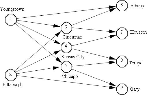 The network represents shipment of finished steel from American Steel's two steel mills located at Youngstown (node 1) and Pittsburgh (node 2) to their field warehouses at Albany, Houston, Tempe, and Gary (nodes 6, 7, 8 and 9) through three regional warehouses located at Cincinnati, Kansas City, and Chicago (nodes 3, 4 and 5). Also, some field warehouses can be directly supplied from the steel mills.
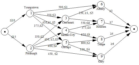
Table 1 presents the minimum and maximum flow amounts of steel that may be shipped between different cities along with the cost per 1000 ton/month of shipping the steel. For example, the shipment from Youngstown to Kansas City is contracted out to a railroad company with a minimal shipping clause of 1000 tons/month. However, the railroad cannot ship more than 5000 tons/month due the shortage of rail cars.
Table 1 Arc Costs and Limits
| From node | To node | Cost | Minimum | Maximum |
| Youngstown | Albany | 500 | - | 1000 |
| Youngstown | Cincinnati | 350 | - | 3000 |
| Youngstown | Kansas City | 450 | 1000 | 5000 |
| Youngstown | Chicago | 375 | - | 5000 |
| Pittsburgh | Cincinnati | 350 | - | 2000 |
| Pittsburgh | Kansas City | 450 | 2000 | 3000 |
| Pittsburgh | Chicago | 400 | - | 4000 |
| Pittsburgh | Gary | 450 | - | 2000 |
| Cincinnati | Albany | 350 | 1000 | 5000 |
| Cincinnati | Houston | 550 | - | 6000 |
| Kansas City | Houston | 375 | - | 4000 |
| Kansas City | Tempe | 650 | - | 4000 |
| Chicago | Tempe | 600 | - | 2000 |
| Chicago | Gary | 120 | - | 4000 |
The current monthly demand at American Steel's four field warehouses is shown in Table 2.
Table 2 Monthly Demands
| Field Warehouses | Monthly Demand |
| Albany, N.Y. | 3000 |
| Houston | 7000 |
| Tempe | 4000 |
| Gary | 6000 |
The Youngstown and Pittsburgh mills can produce up to 10,000 tons and 15,000 tons of steel per month, respectively. The management wants to know the least cost monthly shipment plan.
The network represents shipment of finished steel from American Steel's two steel mills located at Youngstown (node 1) and Pittsburgh (node 2) to their field warehouses at Albany, Houston, Tempe, and Gary (nodes 6, 7, 8 and 9) through three regional warehouses located at Cincinnati, Kansas City, and Chicago (nodes 3, 4 and 5). Also, some field warehouses can be directly supplied from the steel mills.
Table 1 presents the minimum and maximum flow amounts of steel that may be shipped between different cities along with the cost per 1000 ton/month of shipping the steel. For example, the shipment from Youngstown to Kansas City is contracted out to a railroad company with a minimal shipping clause of 1000 tons/month. However, the railroad cannot ship more than 5000 tons/month due the shortage of rail cars.
Table 1 Arc Costs and Limits
| From node | To node | Cost | Minimum | Maximum |
| Youngstown | Albany | 500 | - | 1000 |
| Youngstown | Cincinnati | 350 | - | 3000 |
| Youngstown | Kansas City | 450 | 1000 | 5000 |
| Youngstown | Chicago | 375 | - | 5000 |
| Pittsburgh | Cincinnati | 350 | - | 2000 |
| Pittsburgh | Kansas City | 450 | 2000 | 3000 |
| Pittsburgh | Chicago | 400 | - | 4000 |
| Pittsburgh | Gary | 450 | - | 2000 |
| Cincinnati | Albany | 350 | 1000 | 5000 |
| Cincinnati | Houston | 550 | - | 6000 |
| Kansas City | Houston | 375 | - | 4000 |
| Kansas City | Tempe | 650 | - | 4000 |
| Chicago | Tempe | 600 | - | 2000 |
| Chicago | Gary | 120 | - | 4000 |
The current monthly demand at American Steel's four field warehouses is shown in Table 2.
Table 2 Monthly Demands
| Field Warehouses | Monthly Demand |
| Albany, N.Y. | 3000 |
| Houston | 7000 |
| Tempe | 4000 |
| Gary | 6000 |
The Youngstown and Pittsburgh mills can produce up to 10,000 tons and 15,000 tons of steel per month, respectively. The management wants to know the least cost monthly shipment plan.
|
| ProblemFormulation |
The American Steel Problem can be solved as a transshipment problem. The supply at the supply nodes is the maximum production at the steel mills, i.e., 10,000 and 15,000 for Youngstown and Pittsburgh respectively. The demand at demand nodes in given by the demand at the field warehouses and the other nodes are transshipment nodes. The costs and bounds on flow through the network are also given. The most compact formulation for this problem is a network formulation (see The Transshipment Problem for details).
|
| ComputationalModel |
We can use the AMPL model file transshipment.mod (see The Transshipment Problem in AMPL for details) to solve the American Steel Transshipment Problem. We need a data file to describe the nodes, arcs, costs and bounds. The node set is simply a list of the node names:
set NODES := Youngstown  Pittsburgh
             Cincinnati 'Kansas City' Chicago
             Albany      Houston      Tempe   Gary ;
Note that Kansas City must be enclosed in ' and ' because of the whitespace in the name.
The arc set is 2-dimensional and can be defined in a number of different ways:
# List of arcs
set ARCS := (Youngstown, Albany), (Youngstown, Cincinnati), ... , (Chicago, Gary) ;
# Table of arcs set ARCS: Cincinnati 'Kansas City' Chicago Albany Houston Tempe Gary := Youngstown + + + + - - - Pittsburgh + + + - - - + . . . # Array of arcs set ARCS := (Youngstown, *) Cincinnati 'Kansas City' Chicago Albany (Pittsburgh, *) Cincinnati 'Kansas City' Chicago Gary . . . (Chicago, *) Tempe Gary ;Since the node set is small and the arc set is "dense", i.e., many of the node pairs are represented in the arc set, we choose a table to define ARCS: set ARCS: Cincinnati 'Kansas City' Chicago Albany Houston Tempe Gary := Youngstown + + + + - - - Pittsburgh + + + - - - + Cincinnati - - - + + - - 'Kansas City' - - - - + + - Chicago - - - - - + + ;The NetDemand can be defined easily from the supply and demand. Since the default is 0 we don't need to define NetDemand for the transshipment nodes:
param      NetDemand :=
Youngstown -10000
Pittsburgh -15000
Albany       3000
Houston      7000
Tempe        4000
Gary         6000
 ;
We can use lists, tables or arrays to define the parameters for the American Steel Transhippment Problem, but in this case we will use a list and define multiple parameters at once. This allows us to "cut-and-paste" the parameters from the problem description. Note the use of . for parameters where the defaults will suffice (e.g., Lower for Youngstown and Albany):
param:                  	Cost    Lower  	Upper:=
Youngstown	Albany		500	.	1000
Youngstown	Cincinnati	350	.	3000
Youngstown	'Kansas City'	450	1000	5000
Youngstown	Chicago		375	.	5000
.
.
.
Chicago		Gary		120	.	4000
 ;
Note that the cost is in $/1000 ton, so we must divide the cost by 1000 in our script file before solving:
reset;

model transshipment.mod;

data steel.dat;

let {(m, n) in ARCS} Cost[m, n] := Cost[m, n] / 1000;

option solver cplex;
solve;

display Flow;
We can define the PuLP/Dippy model using functions in transshipment_funcy.py
|
| Results |
Using transshipment.mod, and the data and script files defined in Computational Model we can solve the American Steel Transshipment Problem to get the optimal Flow variables:
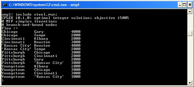 If the total supply is greater than the total demand, the transshipment problem will solve, but flow may be left in the network (in this case at the Pittsburgh node). In
 transshipment.mod we check that sum {n in NODES} NetDemand[n] <= 0 to ensure a problem is feasible before solving.
If total supply is less than demand (hence the problem is infeasible) we can add a dummy supply node (see with arcs to all the demand nodes. The optimal solution will show the "best" nodes to send the extra supply to.
|
| Conclusions |
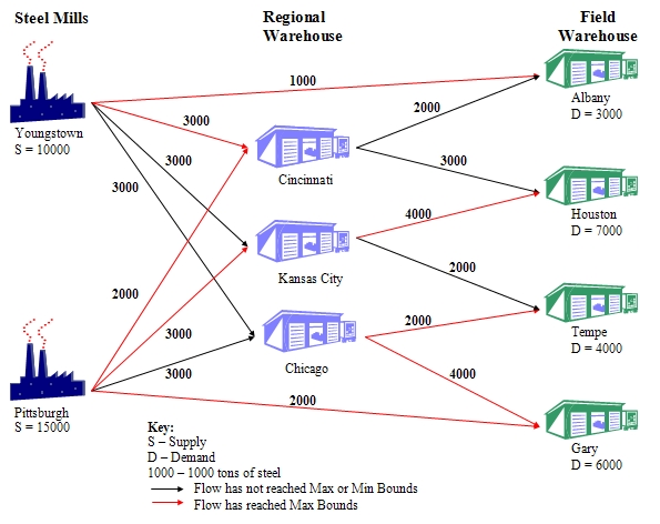
In order to minimise the monthly shipment costs, American Steel should follow the shipment plan shown in Table 3.
Table 3 Optimal Shipment Plan
| From/To | Cincinnati | Kansas City | Chicago | Albany | Houston | Tempe | Gary |
| Youngstown | 3000 | 3000 | 3000 | 1000 | | | |
| Pittsburgh | 2000 | 3000 | 3000 | | | | 2000 |
| Cincinnati | | | | 2000 | 3000 | | |
| Kansas City | | | | | 4000 | 2000 | |
| Chicago | | | | | | 2000 | 4000 |
As with many network problems, it can be illuminating to display the solution graphically as shown in Figure 1.
Figure 1 Optimal Shipment Plan
|
| ExtraForExperts | |
| StudentTasks |
|


Topic revision: r24 - 2014-05-22 - MichaelOSullivan

Ideas, requests, problems regarding TWiki? Send feedback