Difference: CosmicComputersProblem (24 vs. 25)
Revision 252009-10-06 - MichaelOSullivan
| Line: 1 to 1 | ||||||||||||||
|---|---|---|---|---|---|---|---|---|---|---|---|---|---|---|
<-- Ready to Review --> | ||||||||||||||
| Line: 88 to 88 | ||||||||||||||
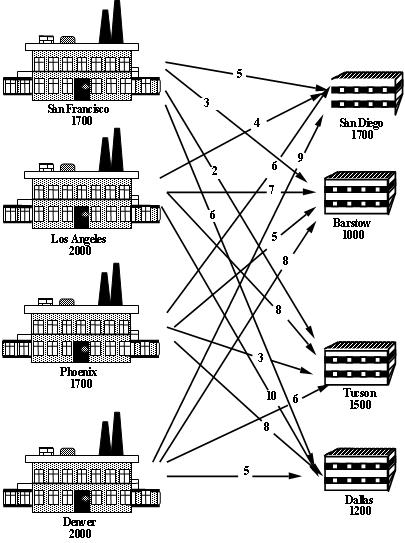 Where should the company set up their plants to minimise their total costs (fixed plus transportation)?
|
|*FORM FIELD ProblemFormulation*|ProblemFormulation|This problem is a facility location problem where the master-slave constraints control the existence of supply nodes for a transportation problem.
Traditional transportation problem formulations are as follows:
Where should the company set up their plants to minimise their total costs (fixed plus transportation)?
|
|*FORM FIELD ProblemFormulation*|ProblemFormulation|This problem is a facility location problem where the master-slave constraints control the existence of supply nodes for a transportation problem.
Traditional transportation problem formulations are as follows:
![\[ \begin{array}{r@{\,}r@{\,}l} \min & \displaystyle \sum_{i \in {\cal S}} \sum_{j \in {\cal D}} c_{ij} & x_{ij} \\ \text{subject to} & \displaystyle \sum_{j \in {\cal D}} & x_{ij} = s_i, i \in {\cal S} \\ & \displaystyle \sum_{i \in {\cal S}} & x_{ij} = d_j, j \in {\cal D} \end{array} \]](/pub/OpsRes/CosmicComputersProblem/latexfb2a6bb240be8ce70a8e2d96e8ceb894.png)
The decisions are two-fold:
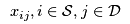 determine where to ship the computers, so we need to add binary variables that govern which of the supply nodes exist, i.e., determine where to ship the computers, so we need to add binary variables that govern which of the supply nodes exist, i.e.,  that are 1 if that are 1 if  exists and 0 otherwise.
2. Formulate the Objective Function exists and 0 otherwise.
2. Formulate the Objective Function
The cost of transporting good through the network is already incorporated into the transportation problem objective, now we have to add the fixed (construction + maintenance) cost
3. Formulate the Constraints
 : :
![\[ \min \sum_{i \in {\cal S}} \sum_{j \in {\cal D}} c_{ij} x_{ij} + \sum_{i \in {\cal S}} C_i z_i \]](/pub/OpsRes/CosmicComputersProblem/latexca3b91b54d0ad3092546d8886c23e7e5.png)
The constraints are the same as the transportation problem formulation, except that the supply is determined by the construction (or not) of a plant:
4. Identify the data
![\[ \sum_{j \in {\cal D}} x_{ij} = s_i z_i, i \in {\cal S} \]](/pub/OpsRes/CosmicComputersProblem/latexa712a9a8cb1360b6b1bfd0763d7d32e3.png) ![\[ \sum_{i \in {\cal S}} x_{ij} \geq d_j, j \in {\cal D} \]](/pub/OpsRes/CosmicComputersProblem/latexcf88a7b42f68cd03fe2a4f8f5621fad3.png)
The data in this problem is the same as that required for a transportation problem, i.e.,
| , ,  , ,  , etc except that the fixed costs also needs to be specified. , etc except that the fixed costs also needs to be specified.
| ||||||||||||||
| Changed: | ||||||||||||||
| < < | |*FORM FIELD ComputationalModel*|ComputationalModel|Since a transportation problem is embedded within the Cosmic Computers Problem, we will start with the AMPl model file transportation.mod (see The Transportation Problem in AMPL for details):
set SUPPLY_NODES;
set DEMAND_NODES;

param Supply {SUPPLY_NODES} >= 0, integer;
param Demand {DEMAND_NODES} >= 0, integer;

param Cost {SUPPLY_NODES, DEMAND_NODES} default 0;

param Lower {SUPPLY_NODES, DEMAND_NODES}
  integer default 0;
param Upper {SUPPLY_NODES, DEMAND_NODES}
  integer default Infinity;

var Flow {i in SUPPLY_NODES, j in DEMAND_NODES}
  >= Lower[i, j], <= Upper[i, j], integer;

minimize TotalCost:
  sum {i in SUPPLY_NODES, j in DEMAND_NODES}
    Cost[i, j] * Flow[i, j];

subject to UseSupply {i in SUPPLY_NODES}:
  sum {j in DEMAND_NODES} Flow[i, j] = Supply[i];

subject to MeetDemand {j in DEMAND_NODES}:
  sum {i in SUPPLY_NODES} Flow[i, j] = Demand[j];
We add new decision variables that decide if we build the production plants or not:
var Build {SUPPLY_NODES} binary;
We define a new parameter for the fixed cost (of construction + maintenance):
param FixedCost {SUPPLY_NODES};
We incorporate the fixed cost into the objective function and the Build variables into the supply constraints and change the supply constraints since the problem may not be balanced:
minimize TotalCost:
  sum {i in SUPPLY_NODES, j in DEMAND_NODES}
    Cost[i, j] * Flow[i, j] +
  sum {i in SUPPLY_NODES} FixedCost[i] * Build[i];

subject to UseSupply {i in SUPPLY_NODES}:
  sum {j in DEMAND_NODES} Flow[i, j] <= Supply[i] * Build[i];
The final model file is given in cosmic.mod.
The data file cosmic.dat is straight forward.
We can also adapt transportation.run by removing all the balancing AMPL commands, e.g., param difference;. We add a different check to cosmic.run that ensures there is enough supply to satisfy the demand (otherwise the problem is infeasible):
check : sum {s in SUPPLY_NODES} Supply[s] >= sum {d in DEMAND_NODES} Demand[d];
| | |||||||||||||
| > > | |*FORM FIELD ComputationalModel*|ComputationalModel|Since a transportation problem is embedded within the Cosmic Computers Problem, we will start with the AMPL model file transportation.mod (see The Transportation Problem in AMPL for details):
set SUPPLY_NODES;
set DEMAND_NODES;

param Supply {SUPPLY_NODES} >= 0, integer;
param Demand {DEMAND_NODES} >= 0, integer;

param Cost {SUPPLY_NODES, DEMAND_NODES} default 0;

param Lower {SUPPLY_NODES, DEMAND_NODES}
  integer default 0;
param Upper {SUPPLY_NODES, DEMAND_NODES}
  integer default Infinity;

var Flow {i in SUPPLY_NODES, j in DEMAND_NODES}
  >= Lower[i, j], <= Upper[i, j], integer;

minimize TotalCost:
  sum {i in SUPPLY_NODES, j in DEMAND_NODES}
    Cost[i, j] * Flow[i, j];

subject to UseSupply {i in SUPPLY_NODES}:
  sum {j in DEMAND_NODES} Flow[i, j] = Supply[i];

subject to MeetDemand {j in DEMAND_NODES}:
  sum {i in SUPPLY_NODES} Flow[i, j] = Demand[j];
We add new decision variables that decide if we build the production plants or not:
var Build {SUPPLY_NODES} binary;
We define a new parameter for the fixed cost (of construction + maintenance):
param FixedCost {SUPPLY_NODES};
We incorporate the fixed cost into the objective function and the Build variables into the supply constraints and change the supply constraints since the problem may not be balanced:
minimize TotalCost:
  sum {i in SUPPLY_NODES, j in DEMAND_NODES}
    Cost[i, j] * Flow[i, j] +
  sum {i in SUPPLY_NODES} FixedCost[i] * Build[i];

subject to UseSupply {i in SUPPLY_NODES}:
  sum {j in DEMAND_NODES} Flow[i, j] <= Supply[i] * Build[i];
The final model file is given in cosmic.mod.
The data file cosmic.dat is straight forward.
We can also adapt transportation.run by removing all the balancing AMPL commands, e.g., param difference;. We add a different check to cosmic.run that ensures there is enough supply to satisfy the demand (otherwise the problem is infeasible):
check : sum {s in SUPPLY_NODES} Supply[s] >= sum {d in DEMAND_NODES} Demand[d];
| | |||||||||||||
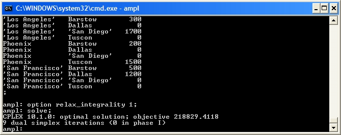
|*FORM FIELD Results*|Results|Using cosmic.run we can solve the Cosmic Computers Problem:
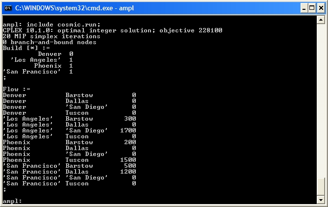 The output shows that CPLEX has not required any branch-and-bound nodes again. Is this problem also naturally integer? We can check by solving the LP relaxation using
 option relax_integrality 1.
 Unfortunately, our problem is not naturally integer. CPLEX performs a lot of "clever tricks" to solve mixed-integer programmes quickly. Let's look at the effect of some of these techniques.
First, we can see what is happening in the branch-and-bound tree by setting the CPLEX options for displaying the branch-and-bound process:
Unfortunately, our problem is not naturally integer. CPLEX performs a lot of "clever tricks" to solve mixed-integer programmes quickly. Let's look at the effect of some of these techniques.
First, we can see what is happening in the branch-and-bound tree by setting the CPLEX options for displaying the branch-and-bound process: mipdisplay 2 gives a moderate amount of information about the process and mipinterval 1 displays this information for every node. For detailed information on setting CPLEX options in AMPL see ILOG's AMPL CPLEX User Guide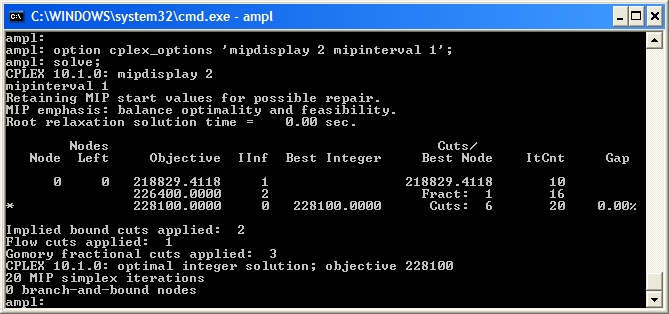 This shows that
 Node 0 (the LP relaxation) is solved, then an integer solution is found quickly with 6 cuts. There are many methods at work here, including:
rinsheur -1 and repairtries -1) and see what happens (Note To see the true effect of these changes you will have to make changes to your script file, restart AMPL and run your script again. Otherwise, AMPL will use your old solution and the effect of your changes will not be obvious):
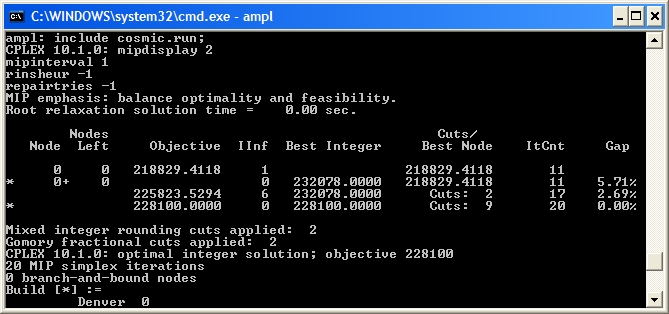 Now the LP relaxation
 Node 0 is solved, but then cuts are generated (indicated by Node 0+) and after 2 cuts are added an integer solution is found, shown by *. After 9 cuts are generated another integer solution is found (hence another *) and this is the optimal solution. Cuts are linear constraints that are added to the LP relaxation to remove fractional solutions. There is a vast amount of literature on cuts for integer programming (try "integer programming cut" on Google), but we will not delve into it here. Let's turn off all the cuts (CPLEX option mipcuts -1) and see what happens:
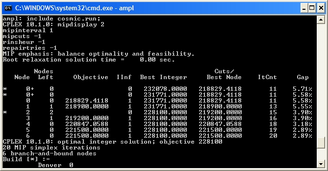 Here the optimal integer solution is found at the second node and then the rest of the tree (6 branch-and-bound nodes in all) is used to ensure this is the optimum. CPLEX is very careful with its selection of a branching variable. Here, it branches on
 Build['Denver'] even though this variable is integer in the LP relaxation. Instead of using the default CPLEX selection rules for the branching variable, let's branch on the fractional variable that is closest to integer (CPLEX option varselect -1):
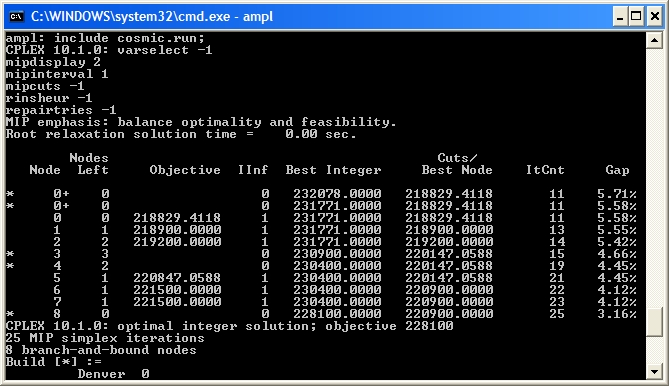 Notice that the branch-and-bound tree is larger (8 nodes as opposed to 6), so this selection strategy did not work as well as the CPLEX default.
While solving the Cosmic Computers Problem we have explored many of the "behind the scenes" work that CPLEX does for you. See Integer Programming with AMPL for more examples. In the Extra for Experts we will see another technique called constraint branching.|
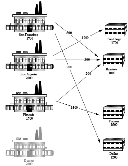
|*FORM FIELD Conclusions*|Conclusions|As with the Brewery Problem, the solution to the Cosmic Computers Problem can be presented in many ways. Figure 1 gives a graphical solution to the Cosmic Computers Problem.
Figure 1 Solution to the Cosmic Computers Problem
Notice that the branch-and-bound tree is larger (8 nodes as opposed to 6), so this selection strategy did not work as well as the CPLEX default.
While solving the Cosmic Computers Problem we have explored many of the "behind the scenes" work that CPLEX does for you. See Integer Programming with AMPL for more examples. In the Extra for Experts we will see another technique called constraint branching.|
|*FORM FIELD Conclusions*|Conclusions|As with the Brewery Problem, the solution to the Cosmic Computers Problem can be presented in many ways. Figure 1 gives a graphical solution to the Cosmic Computers Problem.
Figure 1 Solution to the Cosmic Computers Problem
 |
| | ||||||||||||||
| Changed: | ||||||||||||||
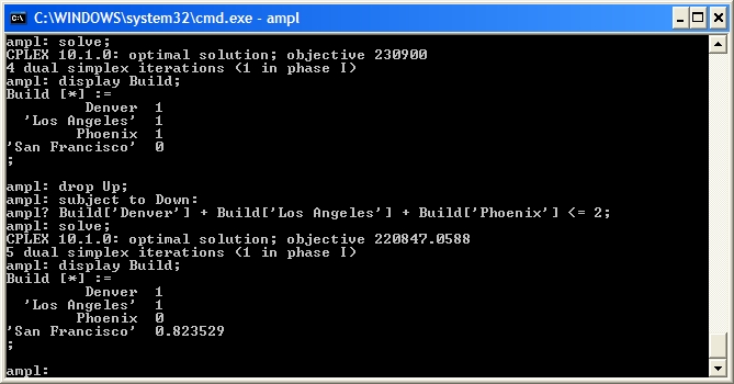
| < < | |*FORM FIELD ExtraForExperts*|ExtraForExperts|Another form of branch and bound implements branches on constraints that should take integer values. For example, in the Cosmic Computers Problem the sum of any subset of Build variables should be integer. Consider the LP relaxation solution:
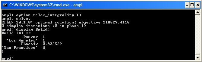 The sum of the three non-zero
 Build variables is 2.82 (2 dp), but it should be integer. We can remove the fractional part by forcing this sum to be either  3 or 3 or  2. First, let's branch up: 2. First, let's branch up:
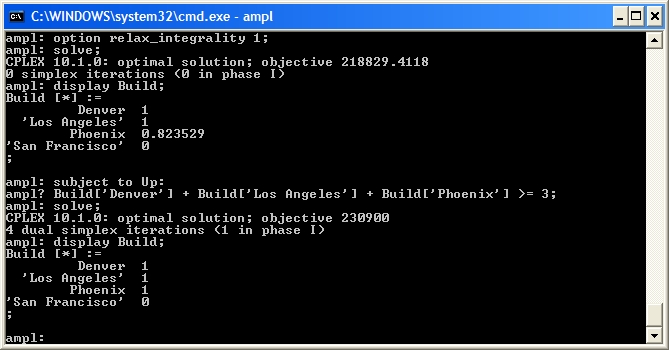 Our solution is integer so we can fathom this node. Now let's drop the Up constraint and branch down:
 This solution still has fractional
 Build variables. We can further constraint branchs to continue searching from this node:
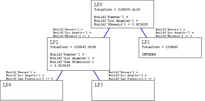 | | | |||||||||||||
| > > | |*FORM FIELD ExtraForExperts*|ExtraForExperts|Another form of branch and bound implements branches on constraints that should take integer values. For example, in the Cosmic Computers Problem the sum of any subset of Build variables should be integer. Consider the LP relaxation solution:
The sum of the three non-zero Build variables is 2.82 (2 dp), but it should be integer. We can remove the fractional part by forcing this sum to be either 3 or 2. First, let's branch up:
Our solution is integer so we can fathom this node. Now let's drop the Up constraint and branch down:
This solution still has fractional Build variables. We can add further constraint branches to continue searching from this node:
| | |||||||||||||
|*FORM FIELD StudentTasks*|StudentTasks|
| ||||||||||||||
View topic | History: r26 < r25 < r24 < r23 | More topic actions...
Ideas, requests, problems regarding TWiki? Send feedback