| CaseStudyForm | |||||||||||||
|---|---|---|---|---|---|---|---|---|---|---|---|---|---|
| Title | Extended Health Clinic | ||||||||||||
| DateSubmitted | 25 Sep 2017 | ||||||||||||
| CaseStudyType | TeachingCaseStudy | ||||||||||||
| OperationsResearchTopics | SimulationModelling | ||||||||||||
| ApplicationAreas | Healthcare | ||||||||||||
| ProblemDescription |
This case study extends the Simple Health Clinic – Scheduled Appointments model. The extensions are:
| ||||||||||||
| ProblemFormulation |
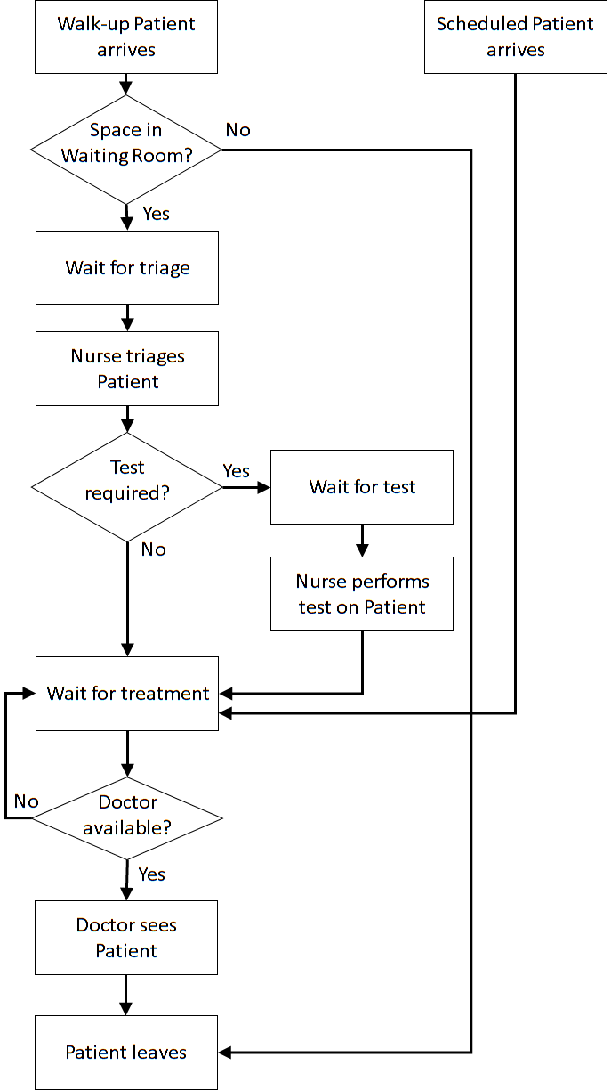
In order to formulate a simulation model we specify the following components:
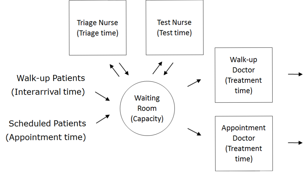
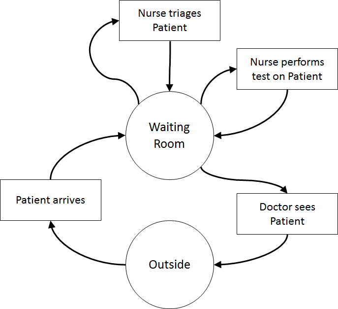 Once the content has been established (note this is usually an iterative process) we can identify the inputs and outputs: appointment times, interarrival times, triage times, test times, treatment times, waiting times for triage, testing, and treatment (i.e., Patient arrives to Nurse triages Patient, Nurse triages Patient to Nurse performs test on Patient, Nurse performs test on Patient to Doctor sees Patient, Nurse triages Patient to Doctor sees Patient, Patient arrives to Doctor sees Patient), total clinic time (Patient arrives to Outside), number in waiting room.
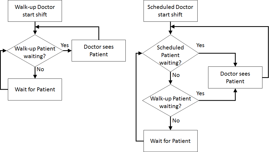
Assumptions are used to define stochasticity (e.g., Exponential interarrivals, Triangular treatment times) and the simplifications keep the system simple (e.g., single doctors and nurses on all day for triage, testing, and treatment, no registration, no prioritisation).
Once the content has been established (note this is usually an iterative process) we can identify the inputs and outputs: appointment times, interarrival times, triage times, test times, treatment times, waiting times for triage, testing, and treatment (i.e., Patient arrives to Nurse triages Patient, Nurse triages Patient to Nurse performs test on Patient, Nurse performs test on Patient to Doctor sees Patient, Nurse triages Patient to Doctor sees Patient, Patient arrives to Doctor sees Patient), total clinic time (Patient arrives to Outside), number in waiting room.
Assumptions are used to define stochasticity (e.g., Exponential interarrivals, Triangular treatment times) and the simplifications keep the system simple (e.g., single doctors and nurses on all day for triage, testing, and treatment, no registration, no prioritisation).
| ||||||||||||
| ComputationalModel |
Start with the Simple Health Clinic – Scheduled Appointments JaamSim model.
 Select the PatientEntity and add a Test attribute to the AttributeDefinitionList by adding { Test 0} to the list.
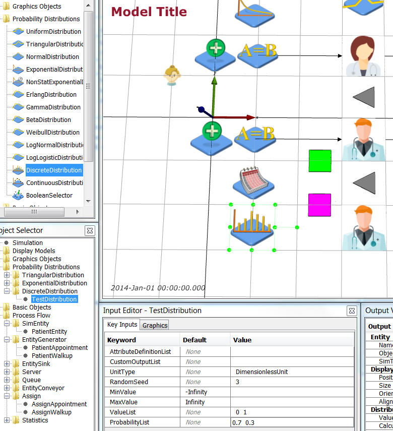
 Now add a distribution that determines if a Walk-Up patient needs a test or not. Add a DiscreteDistribution object from Model Palette > Probability Distributions. Name it TestDistribution and edit it so that 30% of Walk-Up patients require tests.
 | Object | Graphics | Key Inputs |
| TestDistribution | Position = 1 -2.5 0.0 m | UnitType = DimensionlessUnit, ValueList = 0 1, ProbabilityList = 0.7 0.3 |
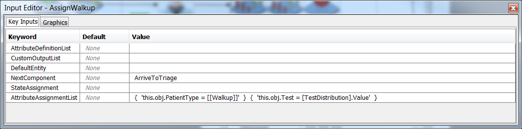
Now select the AssignWalkup object and add {
| Object | Graphics | Key Inputs |
| TestDistribution | Position = 1 -2.5 0.0 m | UnitType = DimensionlessUnit, ValueList = 0 1, ProbabilityList = 0.7 0.3 |
Now select the AssignWalkup object and add { 'this.obj.Test = [TestDistribution].Value' } to AttributeAssignmentList.
 Save your simulation.
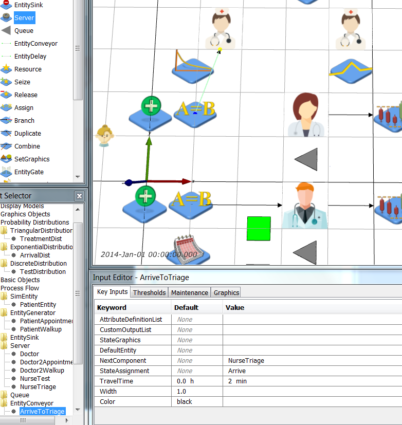
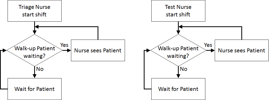
Next, create two new servers (Process Flow > Server), one for triage and one for testing. Name then NurseTriage and NurseTest respectively and give them the nurse.png (icon made by Freepik from www.flaticon.com
Save your simulation.
Next, create two new servers (Process Flow > Server), one for triage and one for testing. Name then NurseTriage and NurseTest respectively and give them the nurse.png (icon made by Freepik from www.flaticon.com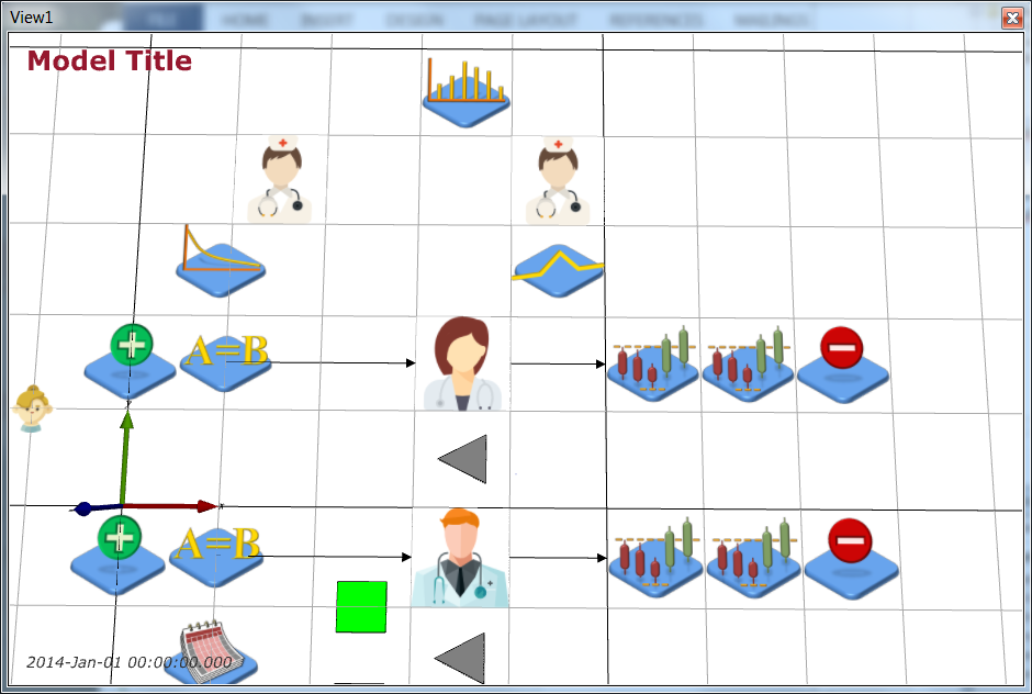 Rename the ArriveToTreat EntityConveyor to be ArriveToTriage and change NextComponent to be NurseTriage. You can redirect the EntityConveyor by clicking on it, then Ctrl-clicking on its end point and dragging it to where you want it to be. Redirect ArriveToTriage as shown below:
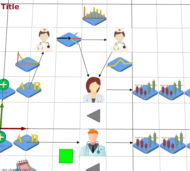
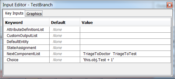
 Next, we need to add the branching for the potential test. Add a Branch object (Model Palette > Process Flow > Branch) and name it TestBranch. Now add 3 more EntityConveyors: TriageToDoctor, TriageToTest, TestToDoctor. TestBranch and the 3 conveyors are shown below (TriageToTest going horizontal left to right, TriageToDoctor diagonally down left, TestToDoctor diagonally down left).
 Next, make sure that the flow of the patients through the triage and test conveyors and servers is set correctly. The TestBranch object uses the value of the entities' Test attribute with 1 added to it to transform it from a {0, 1} value to a {1, 2} value (JaamSim starts lists at 1 not 0), so a patient that doesn't need a test (Test = 0) goes to the first component in the list, i.e., TriageToDoctor conveyor.
 | Object | Key Inputs |
| ArriveToTriage | NextComponent = NurseTriage |
| NurseTriage | NextComponent = TestBranch |
| TestBranch | NextComponentList = TriageToDoctor TriageToTest, Choice =
| Object | Key Inputs |
| ArriveToTriage | NextComponent = NurseTriage |
| NurseTriage | NextComponent = TestBranch |
| TestBranch | NextComponentList = TriageToDoctor TriageToTest, Choice = 'this.obj.Test + 1' |
| TriageToDoctor | NextComponent = Doctor, TravelTime = 2 min |
| TriageToTest | NextComponent = NurseTest, TravelTime = 2 min |
| NurseTest | NextComponent = TestToDoctor |
| TriageToDoctor | NextComponent = Doctor, TravelTime = 2 min |
Save your simulation.
Now, add Queues for both triage and testing, set these queues as the wait queues for triage and testing. The treatment time is modelled by a triangular distribution with minimum 2 minutes, maximum 15 minutes and mode (most likely) 8 minutes, so add a TriangularDistribution called TriageDistribution with these parameters. The test time is modelled as a constant time of 10 minutes, so add this to the NurseTest's ServiceTime. You need to change the StateAssignment of NurseTriage and NurseTest to reflect these activities too.
| Object | Key Inputs |
| NurseTriage | WaitQueue = TriageQueue, StateAssignment = Triage, ServiceTime = TriageDistribution |
| NurseTest | WaitQueue = TestQueue, StateAssignment = Test, ServiceTime = 10 min |
| TriageDistribution | UnitType = TimeUnit, MinValue = 2 min, MaxValue = 15 min, Mode = 8 min |
Finally, you should change the StateAssignment of all your queues so that we can track the time spent waiting for various sets in the pathway. You also need to change the DefaultStateList of your patient entities.
| Object | Key Inputs |
| WalkupQueue | StateAssignment = WaitTreat |
| AppointmentQueue | StateAssignment = WaitTreat |
| TriageQueue | StateAssignment = WaitTriage |
| TestQueue | StateAssignment = WaitTest |
| PatientEntity | DefaultStateList = { Arrive WaitTreat WaitTriage WaitTest Treat Triage Test Leave } |
Save your simulation.
At this point you can run your simulation and ensure that your triage/test process does not cause any errors.
However, now that the PatientEntity has new states we need to modify and append our Statistics modules and Simulation output. Change the existing Statistics modules to gather all the time in the system and waiting times and change the outputs generated by the simulation.
| Object | Key Inputs |
| TimeInSystem | SampleValue = 'this.obj.StateTimes([[Arrive]]) + this.obj.StateTimes([[WaitTriage]]) + this.obj.StateTimes([[Triage]]) + this.obj.StateTimes([[WaitTest]]) + this.obj.StateTimes([[Test]]) + this.obj.StateTimes([[WaitTreat]]) + this.obj.StateTimes([[Treat]]) + this.obj.StateTimes([[Leave]])' |
| WaitingTime | NextComponent = WaitingTriage SampleValue = 'this.obj.StateTimes([[WaitTriage]]) + this.obj.StateTimes([[WaitTest]]) + this.obj.StateTimes([[WaitTreat]])' |
| TimeInSystem2 | SampleValue = 'this.obj.StateTimes([[Arrive]]) + this.obj.StateTimes([[WaitTreat]]) + this.obj.StateTimes([[Treat]]) + this.obj.StateTimes([[Leave]])' |
| WaitingTime2 | NextComponent = WaitingTriage SampleValue = this.obj.StateTimes([[WaitTreat]]) | | WaitingTriage (New Statistics component) | UnitType = TimeUnit NextComponent = WaitingTest SampleValue = this.obj.StateTimes([[WaitTriage]]) | | WaitingTest (New Statistics component) | UnitType = TimeUnit NextComponent = WaitingTreat SampleValue = this.obj.StateTimes([[WaitTest]]) | | WaitingTreat (New Statistics component) | UnitType = TimeUnit NextComponent = PatientWalkupSink SampleValue = this.obj.StateTimes([[WaitTreat]]) | | Simulation | UnitTypeList = DimensionlessUnit TimeUnit TimeUnit TimeUnit TimeUnit TimeUnit DimensionlessUnit DimensionlessUnit TimeUnit TimeUnit DimensionlessUnit DimensionlessUnit RunOutputList = { [Simulation].RunIndex(1) } { [WaitingTriage].SampleAverage } { [WaitingTest].SampleAverage } { [WaitingTreat].SampleAverage } { [WaitingTime].SampleAverage } { [TimeInSystem].SampleAverage } { [WalkupQueue].QueueLengthAverage } { [Doctor].Utilisation } { [WaitingTime2].SampleAverage } { [TimeInSystem2].SampleAverage } { [AppointmentQueue].QueueLengthAverage } { '[Doctor2Appointment].Utilisation + [Doctor2Walkup].Utilisation' } |
Save your simulation.
Run your simulation and use Lab3Analysis.R to look at the results from your simulation with the triage and tests added. The confidence intervals results should look as follows:
| Measure | WalkUp.WaitingTriage | WalkUp.WaitingTest | WalkUp.WaitingTreat | WalkUp.WaitingTime | WalkUp.TimeInSystem | WalkUp.Queue | Doctor.Utilisation | Appointment.WaitingTime | Appointment.TimeInSystem | Appointment.Queue | Doctor2.Utilisation |
| ConfLower | 0.05288071 | 0.001722233 | 0.1299629 | 0.1856799 | 0.6999984 | 0.5610395 | 0.6138156 | 0.1187734 | 0.3684660 | 0.3531135 | 0.8678660 |
| Mean | 0.05454892 | 0.001860125 | 0.1365626 | 0.1929717 | 0.7079008 | 0.5866481 | 0.6196521 | 0.1210310 | 0.3711808 | 0.3598717 | 0.8705052 |
| ConfUpper | 0.05621712 | 0.001998017 | 0.1431624 | 0.2002634 | 0.7158032 | 0.6122568 | 0.6254886 | 0.1232887 | 0.3738955 | 0.3666299 | 0.8731443 |
By contrast, the final results from SHC with Scheduled Appointments are:
| RunNumber | WalkUp.WaitingTime | WalkUp.TimeInSystem | WalkUp.Queue | Doctor.Utilisation | Appointment.WaitingTime | Appointment.TimeInSystem | Appointment.Queue | Doctor2.Utilisation |
| 4 | 0.1592253 | 0.4426042 | 0.4840191 | 0.6174519 | 0.12180412 | 0.4048019 | 0.3623689 | 0.8726559 |
| RunNumber | Quantity | WalkUp.WaitingTime | WalkUp.TimeInSystem | WalkUp.Queue | Doctor.Utilisation | Appointment.WaitingTime | Appointment.TimeInSystem | Appointment.Queue | Doctor2.Utilisation |
| 4 | .1 | 0.1521349 | 0.4352098 | 0.4599628 | 0.6113834 | 0.11939828 | 0.4019517 | 0.3552248 | 0.8703043 |
| | .2 | 0.1663157 | 0.4499985 | 0.5080754 | 0.6235204 | 0.12420996 | 0.4076520 | 0.369513 | 0.8750076 |
Hence, the walk-up patients are worse off because of the extras steps in their pathways, but the appointment patients are a little better off with the triage and testing process in place. This make sense as the flow of walk-up patients to the doctors has been "stretched" by the triage and testing process, so less walk-up patients will be able to take advantage of any gaps in the appointment schedule and less appointment patients will get delayed by walk-up patients utilising the doctor for appointment patients.
Next, we add some uncertainty to the arrival time of appointment patients by adding a little "noise" to their arrival. Create a NormalDistribution object called AppointmentDistribution with mean 0 minutes, standard deviation 5 minutes and minimum value -15 minutes (this will "truncate" the negative tail of the distribution. Add the value from this distribution to the AppointmentTimes value in the PatientAppointment EntityGenerator.
| Object | Key Inputs |
| AppointmentDistribution | UnitType = TimeUnit MinValue = -15 min Mean = 0 min StandardDeviation = 5 min | | PatientAppointment | FirstArrivalTime = '[AppointmentTimes].Value + [AppointmentDistribution].Value' InterArrivalTime = '[AppointmentTimes].Value + [AppointmentDistribution].Value' |
Save your simulation.
Re-run your simulation and see what effect the appointment time "noise" has. Here is the doctor utilisation and appointment patients' statistics:
| Measure | Doctor.Utilisation | Appointment.WaitingTime | Appointment.TimeInSystem | Appointment.Queue | Doctor2.Utilisation |
| ConfLower | 0.6156018 | 0.1411374 | 0.3908679 | 0.4184674 | 0.8658708 |
| Mean | 0.6214994 | 0.1441949 | 0.3943305 | 0.4278683 | 0.8685447 |
| ConfUpper | 0.6273969 | 0.1472523 | 0.3977932 | 0.4372693 | 0.8712186 |
Finally, we add some non-stationarity to the arrival rate of the walk-up patients. Add a TimeSeries object call WalkupRates to define the changing arrival rates of walk-up patients. Suppose we want an arrival process with exponentially distributed interarrival times with mean 1 hour between midnight and 8 a.m. (8 arrivals expected), mean 15 mins between 8 a.m. and 5 p.m. (36 arrivals expected), and mean 30 mins between 5 p.m. and midnight (14 arrivals expected). We would edit WalkupRates to define the number that arrived over time as follows:
| Object | Key Inputs |
| WalkupRates | UnitType = DimensionlessUnit Value = {0 h 0} {8 h 8} {17 h 44} {24 h 58} CycleTime = 24 h | This means that at 0 hrs, 0 have arrived, at 8 hrs 8 have arrived, at 17 hrs 44 ( 8 + 36) have arrived, and at 24 hrs 58 ( 8 + 36 + 14) have arrived.
Add a NonStatExponentialDistribution called WalkupDistribution to your model that uses WalkupRates to generate arrivals:
| Object | Key Inputs |
| WalkupDistribution | ExpectedArrivals = WalkupRates |
Lastly, use WalkupDistribution to define the first and inter arrivals times in the PatientWalkup EntityGenerator.
| Object | Key Inputs |
| PatientWalkup | FirstArrivalTime = '([Simulation].RunIndex(1) == 1) || ([Simulation].RunIndex(1) == 3) ? 20[min] : [WalkupDistribution].Value' InterArrivalTime = '([Simulation].RunIndex(1) == 1) || ([Simulation].RunIndex(1) == 3) ? 20[min] : [WalkupDistribution].Value' |
Save your simulation.
| ||||||||||||
| Results |
As in SHC with Scheduled Appointments, perform 100 runs of this simulation each 168 hours long and with 24 hours warm up to examine the effect of the changes to the health clinic and observe the difference in average time in system and queue length for the walk up and appointment patients, and the difference in utilisation of the walk up only doctor and the appointment and walk up doctor. No changes to the Simulation object’s Key Inputs other than those described earlier in this case study are needed. The Simulation runs are as follows:
| Object | Multiple Runs | Value |
| Simulation | RunIndexDefinitionList | 4 100 |
| | StartingRunNumber | 4-1 |
| | EndingRunNumber | 4-100 |
Run your simulation and modify Lab3Analysis.R to use your new .dat file. Your results should be as below.
          WalkUp.WaitingTriage WalkUp.WaitingTest WalkUp.WaitingTreat
ConfLower           0.06348941        0.001782069           0.1691806
Mean                0.06669406        0.001939454           0.1821196
ConfUpper           0.06989872        0.002096840           0.1950587
          WalkUp.WaitingTime WalkUp.TimeInSystem WalkUp.Queue
ConfLower          0.2358568           0.7504917    0.5717737
Mean               0.2507531           0.7657013    0.6116139
ConfUpper          0.2656495           0.7809109    0.6514542
          Doctor.Utilisation Appointment.WaitingTime Appointment.TimeInSystem
ConfLower          0.4939916               0.1247468                0.3747652
Mean               0.4992751               0.1274355                0.3779698
ConfUpper          0.5045585               0.1301242                0.3811744
          Appointment.Queue Doctor2.Utilisation
ConfLower         0.3695416           0.8397049
Mean              0.3779435           0.8426485
ConfUpper         0.3863453           0.8455921
ValueTraceList = { '[TriageQueue].QueueLength + [TestQueue].QueueLength + [WalkupQueue].QueueLength + [AppointmentQueue].QueueLength' } |
Now adapt parse_multiple_runs_log.R to draw the number in the waiting room for the first 10 replications (note that parse_single_run_log.R is also attached for your reference). The plot should look like:
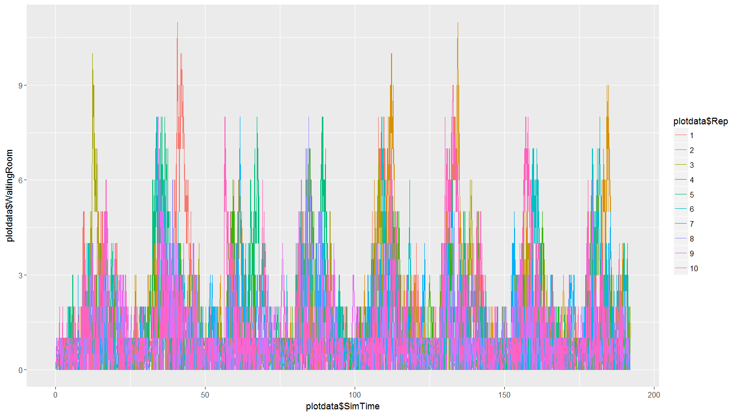 Note the cyclical nature of the plot that demonstrates the daily effect of the variable arrival rates for walk-up patients.
| ||||||||||||
| Conclusions | In this case study, you extended the SHC with Scheduled Appointments models to a triage/testing process, "noise" on appointment patient arrivals, and non-stationary arrival rates for walk-up patients. You investigated the effect of the changes as well as plotting the number in the waiting room over time to see the effect of non-stationarity. Given the imbalance between the utilisation of the doctors, how should the two doctors be rostered to ensure their workload is equitable? | ||||||||||||
| ExtraForExperts | |||||||||||||
| StudentTasks | |||||||||||||


| I | Attachment | History | Action | Size | Date | Who | Comment |
|---|---|---|---|---|---|---|---|
| |
Lab3Analysis.R | r1 | manage | 1.7 K | 2017-09-28 - 04:05 | MichaelOSullivan | |
| |
nurse.png | r1 | manage | 5.1 K | 2017-09-28 - 02:44 | MichaelOSullivan | |
| |
parse_multiple_runs_log.R | r1 | manage | 2.1 K | 2017-09-29 - 02:38 | MichaelOSullivan | |
| |
parse_single_run_log.R | r1 | manage | 2.0 K | 2017-09-29 - 02:38 | MichaelOSullivan |
This topic: OpsRes > SubmitCaseStudy > ExtendedHealthClinic
Topic revision: r7 - 2017-09-29 - MichaelOSullivan
Ideas, requests, problems regarding TWiki? Send feedback