Case Study: Extended Health Clinic
Submitted: 25 Sep 2017
Operations Research Topics: SimulationModelling
Application Areas: Healthcare
Contents
Problem Description
This case study extends the Simple Health Clinic – Scheduled Appointments model. The extensions are:- Walk-up patients are triaged before receiving treatment;
- After being triaged, some walk-up patients need to have a test performed before seeing a doctor;
- Appointment patients arrive at their appointment times +/- a few minutes;
- The arrival rate of walk-up patients varies over the day.
- waiting for treatment; and
- in the clinic;
Problem Formulation
In order to formulate a simulation model we specify the following components:- Background – problem description
- Objectives of the study
- Expected benefits
- The CM: inputs, outputs, content, assumptions, simplifications’
- Experiments to run
- Component List
- Process flow diagram
- Logic flow diagram
- Activity cycle diagram
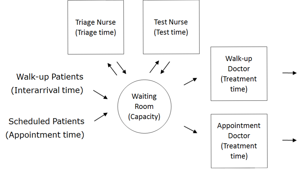
- Walk-up patients with their (inter)arrival times
- Scheduled patients with their appointment times
- Triage nurses with their triage times
- Test nurses with their testing times
- Doctors with their treatment times
- Waiting room with its capacity
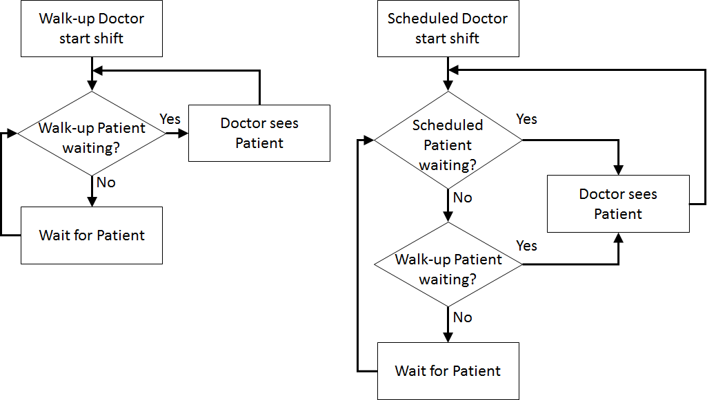
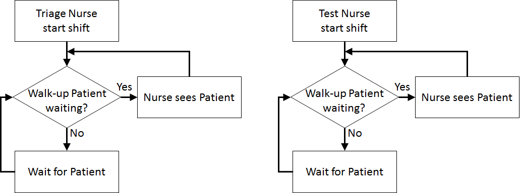
| Patient Logic Flow Diagram | Doctor Logic Flow Diagrams | |
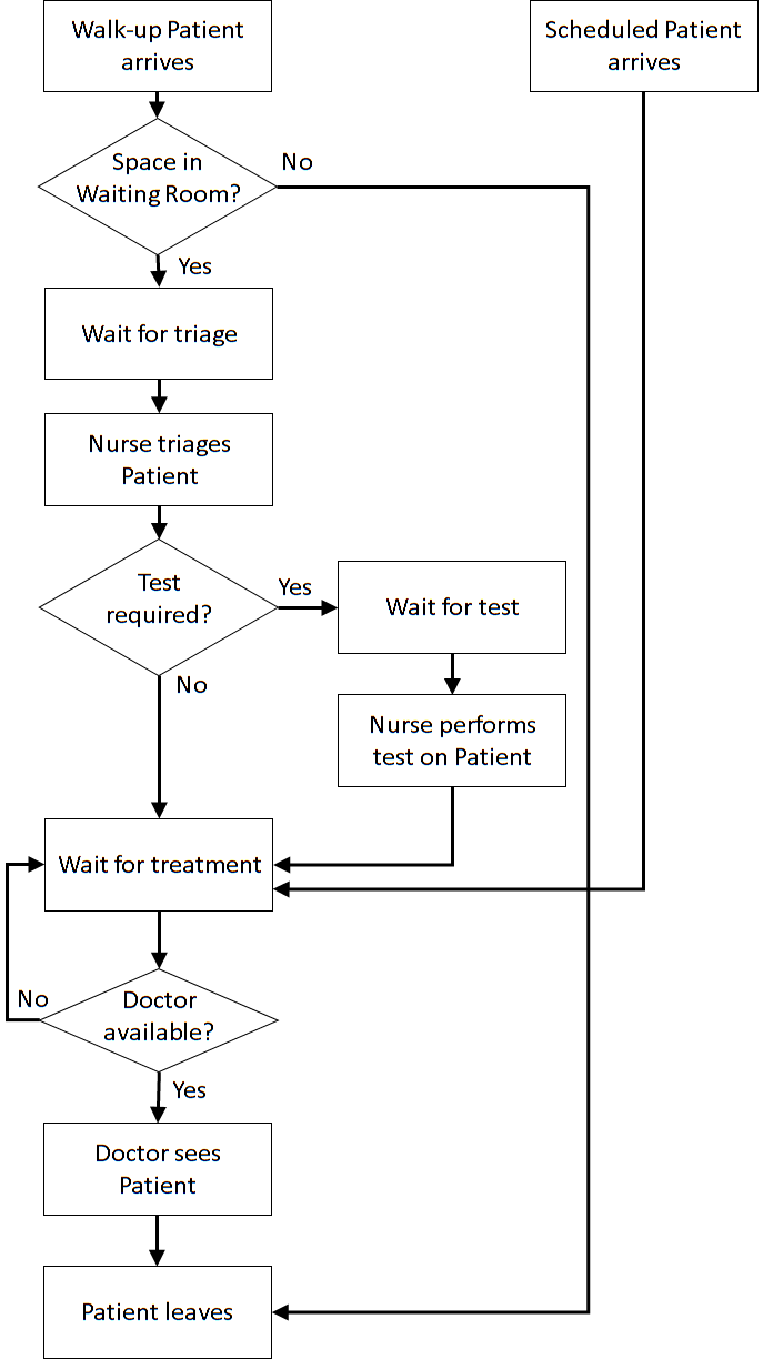 |  | |
| Nurse Logic Flow Diagrams | ||
 | ||
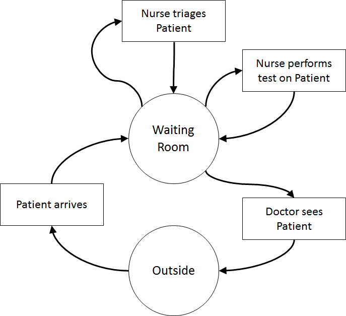 Once the content has been established (note this is usually an iterative process) we can identify the inputs and outputs: appointment times, interarrival times, triage times, test times, treatment times, waiting times for triage, testing, and treatment (i.e., Patient arrives to Nurse triages Patient, Nurse triages Patient to Nurse performs test on Patient, Nurse performs test on Patient to Doctor sees Patient, Nurse triages Patient to Doctor sees Patient, Patient arrives to Doctor sees Patient), total clinic time (Patient arrives to Outside), number in waiting room.
Assumptions are used to define stochasticity (e.g., Exponential interarrivals, Triangular treatment times) and the simplifications keep the system simple (e.g., single doctors and nurses on all day for triage, testing, and treatment, no registration, no prioritisation).
Return to top
Once the content has been established (note this is usually an iterative process) we can identify the inputs and outputs: appointment times, interarrival times, triage times, test times, treatment times, waiting times for triage, testing, and treatment (i.e., Patient arrives to Nurse triages Patient, Nurse triages Patient to Nurse performs test on Patient, Nurse performs test on Patient to Doctor sees Patient, Nurse triages Patient to Doctor sees Patient, Patient arrives to Doctor sees Patient), total clinic time (Patient arrives to Outside), number in waiting room.
Assumptions are used to define stochasticity (e.g., Exponential interarrivals, Triangular treatment times) and the simplifications keep the system simple (e.g., single doctors and nurses on all day for triage, testing, and treatment, no registration, no prioritisation).
Return to top
Computational Model
Start with the Simple Health Clinic – Scheduled Appointments JaamSim model.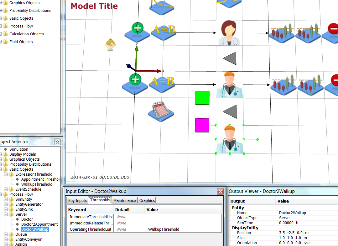 Select the PatientEntity and add a Test attribute to the AttributeDefinitionList by adding { Test 0} to the list.
 Now add a distribution that determines if a Walk-Up patient needs a test or not. Add a DiscreteDistribution object from Model Palette > Probability Distributions. Name it TestDistribution and edit it so that 30% of Walk-Up patients require tests.
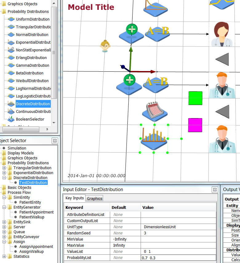
| Object | Graphics | Key Inputs |
|---|---|---|
| TestDistribution | Position = 1 -2.5 0.0 m | UnitType = DimensionlessUnit, RandomSeed = 3, ValueList = 0 1, ProbabilityList = 0.7 0.3 |
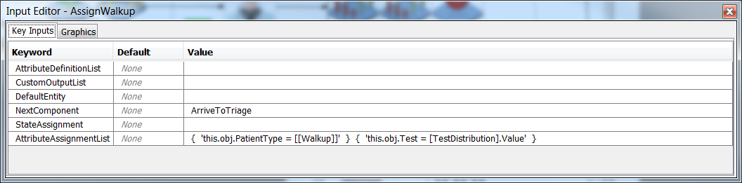
'this.obj.Test = [TestDistribution].Value' } to AttributeAssignmentList.
 Save your simulation.
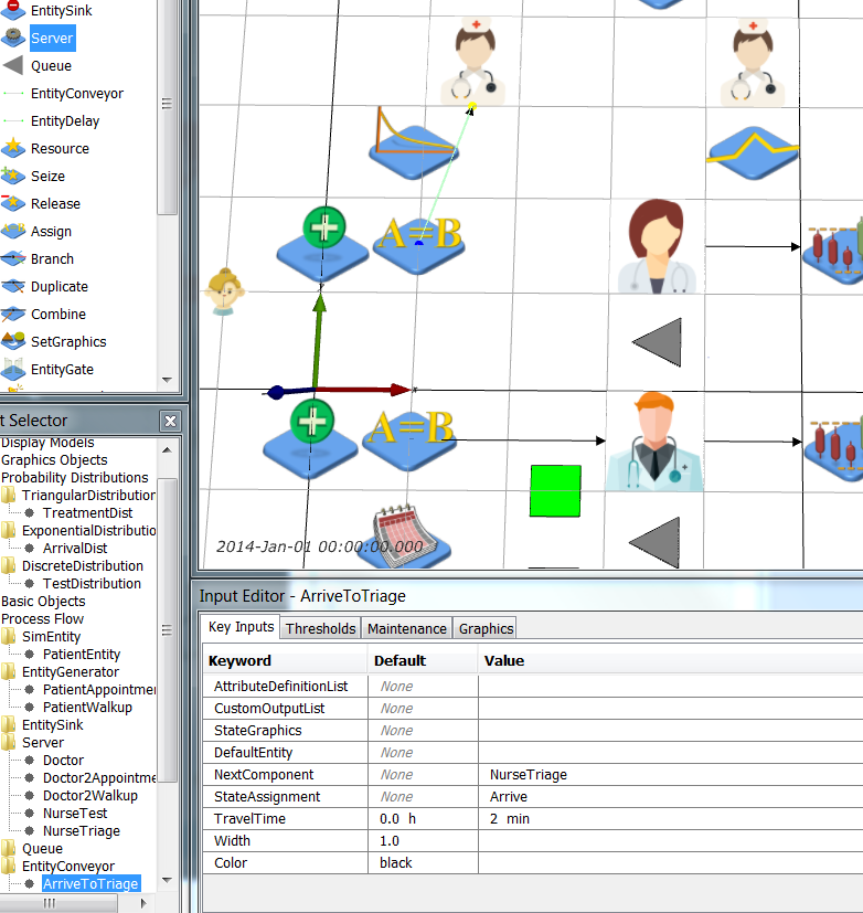
Next, create two new servers (Process Flow > Server), one for triage and one for testing. Name then NurseTriage and NurseTest respectively and give them the nurse.png (icon made by Freepik from www.flaticon.com
Save your simulation.
Next, create two new servers (Process Flow > Server), one for triage and one for testing. Name then NurseTriage and NurseTest respectively and give them the nurse.png (icon made by Freepik from www.flaticon.com Rename the ArriveToTreat EntityConveyor to be ArriveToTriage and change NextComponent to be NurseTriage. You can redirect the EntityConveyor by clicking on it, then Ctrl-clicking on its end point and dragging it to where you want it to be. Redirect ArriveToTriage as shown below:
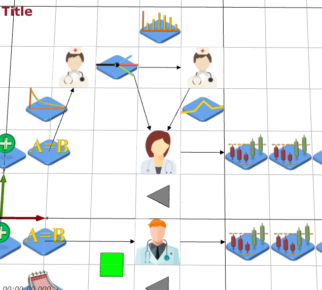
 Next, we need to add the branching for the potential test. Add a Branch object (Model Palette > Process Flow > Branch) and name it TestBranch. Now add 3 more EntityConveyors: TriageToDoctor, TriageToTest, TestToDoctor. TestBranch and the 3 conveyors are shown below (TriageToTest going horizontal left to right, TriageToDoctor diagonally down left, TestToDoctor diagonally down left).
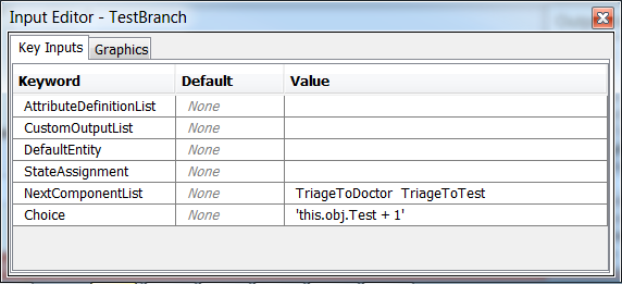
 Next, make sure that the flow of the patients through the triage and test conveyors and servers is set correctly. The TestBranch object uses the value of the entities' Test attribute with 1 added to it to transform it from a {0, 1} value to a {1, 2} value (JaamSim starts lists at 1 not 0), so a patient that doesn't need a test (Test = 0) goes to the first component in the list, i.e., TriageToDoctor conveyor.
| Object | Key Inputs |
|---|---|
| ArriveToTriage | NextComponent = NurseTriage |
| NurseTriage | NextComponent = TestBranch |
| TestBranch | NextComponentList = TriageToDoctor TriageToTest, Choice = 'this.obj.Test + 1' |
| TriageToDoctor | NextComponent = Doctor, TravelTime = 2 min |
| TriageToTest | NextComponent = NurseTest, TravelTime = 2 min |
| NurseTest | NextComponent = TestToDoctor |
| TestToDoctor | NextComponent = Doctor, TravelTime = 2 min |
| Object | Key Inputs |
|---|---|
| NurseTriage | WaitQueue = TriageQueue, StateAssignment = Triage, ServiceTime = TriageDistribution |
| NurseTest | WaitQueue = TestQueue, StateAssignment = Test, ServiceTime = 10 min |
| TriageDistribution | UnitType = TimeUnit, RandomSeed = 4, MinValue = 2 min, MaxValue = 15 min, Mode = 8 min |
| Object | Key Inputs |
|---|---|
| WalkupQueue | StateAssignment = WaitTreat |
| AppointmentQueue | StateAssignment = WaitTreat |
| TriageQueue | StateAssignment = WaitTriage |
| TestQueue | StateAssignment = WaitTest |
| PatientEntity | DefaultStateList = { Arrive WaitTreat WaitTriage WaitTest Treat Triage Test Leave } |
| Object | Key Inputs |
|---|---|
| TimeInSystem | SampleValue = 'this.obj.StateTimes("Arrive") + this.obj.StateTimes("WaitTriage") + this.obj.StateTimes("Triage") + this.obj.StateTimes("WaitTest") + this.obj.StateTimes("Test") + this.obj.StateTimes("WaitTreat") + this.obj.StateTimes("Treat") + this.obj.StateTimes("Leave")' |
| WaitingTime | NextComponent = WaitingTriage SampleValue = 'this.obj.StateTimes("WaitTriage") + this.obj.StateTimes("WaitTest") + this.obj.StateTimes("WaitTreat")' |
| TimeInSystem2 | SampleValue = 'this.obj.StateTimes("Arrive") + this.obj.StateTimes("WaitTreat") + this.obj.StateTimes("Treat") + this.obj.StateTimes("Leave")' |
| WaitingTime2 | SampleValue = this.obj.StateTimes("WaitTreat") |
| WaitingTriage (New Statistics component) | UnitType = TimeUnit NextComponent = WaitingTest SampleValue = this.obj.StateTimes("WaitTriage") |
| WaitingTest (New Statistics component) | UnitType = TimeUnit NextComponent = WaitingTreat SampleValue = this.obj.StateTimes("WaitTest") |
| WaitingTreat (New Statistics component) | UnitType = TimeUnit NextComponent = PatientWalkupSink SampleValue = this.obj.StateTimes("WaitTreat") |
| Simulation | UnitTypeList = DimensionlessUnit TimeUnit TimeUnit TimeUnit TimeUnit TimeUnit DimensionlessUnit DimensionlessUnit TimeUnit TimeUnit DimensionlessUnit DimensionlessUnit RunOutputList = { [Simulation].RunIndex(1) } { [WaitingTriage].SampleAverage } { [WaitingTest].SampleAverage } { [WaitingTreat].SampleAverage } { [WaitingTime].SampleAverage } { [TimeInSystem].SampleAverage } { '[TriageQueue].QueueLengthAverage + [TestQueue].QueueLengthAverage + [WalkupQueue].QueueLengthAverage' } { [Doctor].Utilisation } { [WaitingTime2].SampleAverage } { [TimeInSystem2].SampleAverage } { [AppointmentQueue].QueueLengthAverage } { '[Doctor2Appointment].Utilisation + [Doctor2Walkup].Utilisation' } |
| Measure | WalkUp.WaitingTriage | WalkUp.WaitingTest | WalkUp.WaitingTreat | WalkUp.WaitingTime | WalkUp.TimeInSystem | Num.WalkUps.Waiting | Doctor.Utilisation | Appointment.WaitingTime | Appointment.TimeInSystem | Appointment.Queue | Doctor2.Utilisation |
|---|---|---|---|---|---|---|---|---|---|---|---|
| ConfLower | 0.05326031 | 0.001735700 | 0.1304301 | 0.1865163 | 0.7018218 | 0.5606735 | 0.6132686 | 0.1192807 | 0.4022488 | 0.3524806 | 0.8683465 |
| Mean | 0.05493219 | 0.001873389 | 0.1371880 | 0.1939935 | 0.7099500 | 0.5865928 | 0.6191527 | 0.1215904 | 0.4050244 | 0.3593692 | 0.8709183 |
| ConfUpper | 0.05660406 | 0.002011078 | 0.1439458 | 0.2014707 | 0.7180781 | 0.6125121 | 0.6250368 | 0.1239000 | 0.4078001 | 0.3662577 | 0.8734901 |
| RunNumber | WalkUp.WaitingTime | WalkUp.TimeInSystem | WalkUp.Queue | Doctor.Utilisation | Appointment.WaitingTime | Appointment.TimeInSystem | Appointment.Queue | Doctor2.Utilisation |
|---|---|---|---|---|---|---|---|---|
| 4 | 0.1592253 | 0.4426042 | 0.4840191 | 0.6174519 | 0.12180412 | 0.4048019 | 0.3623689 | 0.8726559 |
| RunNumber | Quantity | WalkUp.WaitingTime | WalkUp.TimeInSystem | WalkUp.Queue | Doctor.Utilisation | Appointment.WaitingTime | Appointment.TimeInSystem | Appointment.Queue | Doctor2.Utilisation |
|---|---|---|---|---|---|---|---|---|---|
| 4 | .1 | 0.1521349 | 0.4352098 | 0.4599628 | 0.6113834 | 0.11939828 | 0.4019517 | 0.3552248 | 0.8703043 |
| .2 | 0.1663157 | 0.4499985 | 0.5080754 | 0.6235204 | 0.12420996 | 0.4076520 | 0.369513 | 0.8750076 |
| Object | Key Inputs |
|---|---|
| AppointmentDistribution | UnitType = TimeUnit RandomSeed = 5 MinValue = -15 min Mean = 0 min StandardDeviation = 5 min |
| PatientAppointment | FirstArrivalTime = '[AppointmentTimes].Value + [AppointmentDistribution].Value' InterArrivalTime = '[AppointmentTimes].Value + [AppointmentDistribution].Value' |
| Measure | Doctor.Utilisation | Appointment.WaitingTime | Appointment.TimeInSystem | Appointment.Queue | Doctor2.Utilisation |
|---|---|---|---|---|---|
| ConfLower | 0.6166581 | 0.1414877 | 0.4241283 | 0.4174881 | 0.8646724 |
| Mean | 0.6225270 | 0.1446245 | 0.4277147 | 0.4270835 | 0.8675022 |
| ConfUpper | 0.6283959 | 0.1477613 | 0.4313011 | 0.4366789 | 0.8703320 |
| Object | Key Inputs |
|---|---|
| WalkupRates | UnitType = DimensionlessUnit Value = {0 h 0} {8 h 8} {17 h 44} {24 h 58} CycleTime = 24 h |
8 + 36) have arrived, and at 24 hrs 58 ( 8 + 36 + 14) have arrived.
Add a NonStatExponentialDistribution called WalkupDistribution to your model that uses WalkupRates to generate arrivals:
| Object | Key Inputs |
|---|---|
| WalkupDistribution | ExpectedArrivals = WalkupRates |
| Object | Key Inputs |
|---|---|
| PatientWalkup | FirstArrivalTime = '([Simulation].RunIndex(1) == 1) || ([Simulation].RunIndex(1) == 3) ? 20[min] : [WalkupDistribution].Value' InterArrivalTime = '([Simulation].RunIndex(1) == 1) || ([Simulation].RunIndex(1) == 3) ? 20[min] : [WalkupDistribution].Value' |
Results
As in SHC with Scheduled Appointments, perform 100 runs of this simulation each 168 hours long and with 24 hours warm up to examine the effect of the changes to the health clinic and observe the difference in average time in system and queue length for the walk up and appointment patients, and the difference in utilisation of the walk up only doctor and the appointment and walk up doctor. No changes to the Simulation object’s Key Inputs other than those described earlier in this case study are needed. The Simulation runs are as follows:| Object | Multiple Runs | Value |
|---|---|---|
| Simulation | RunIndexDefinitionList | 4 100 |
| StartingRunNumber | 4-1 | |
| EndingRunNumber | 4-100 |
          WalkUp.WaitingTriage WalkUp.WaitingTest WalkUp.WaitingTreat
ConfLower           0.06360199        0.001792959           0.1694404
Mean                0.06682758        0.001953419           0.1824697
ConfUpper           0.07005316        0.002113880           0.1954990
          WalkUp.WaitingTime WalkUp.TimeInSystem Num.WalkUps.Waiting
ConfLower          0.2362326           0.7518122       0.5720433
Mean               0.2512507           0.7671848       0.6122041
ConfUpper          0.2662688           0.7825573       0.6523649
          Doctor.Utilisation Appointment.WaitingTime Appointment.TimeInSystem
ConfLower          0.4941766               0.1261258                0.4090825
Mean               0.4993517               0.1292271                0.4126293
ConfUpper          0.5045268               0.1323284                0.4161760
          Appointment.Queue Doctor2.Utilisation
ConfLower         0.3721434           0.8395105
Mean              0.3817525           0.8425352
ConfUpper         0.3913617           0.8455598
> t.test(Lab3scen$WalkUp.WaitingTime, Lab3scen$Appointment.WaitingTime)

        Welch Two Sample t-test

data:  Lab3scen$WalkUp.WaitingTime and Lab3scen$Appointment.WaitingTime
t = 15.789, df = 107.43, p-value < 2.2e-16
alternative hypothesis: true difference in means is not equal to 0
95 percent confidence interval:
 0.1067035 0.1373437
sample estimates:
mean of x mean of y
0.2512507 0.1292271
|
> t.test(Lab3scen$WalkUp.TimeInSystem, Lab3scen$Appointment.TimeInSystem)

        Welch Two Sample t-test

data:  Lab3scen$WalkUp.TimeInSystem and Lab3scen$Appointment.TimeInSystem
t = 44.593, df = 110.3, p-value < 2.2e-16
alternative hypothesis: true difference in means is not equal to 0
95 percent confidence interval:
 0.3387978 0.3703132
sample estimates:
mean of x mean of y
0.7671848 0.4126293
|
> t.test(Lab3scen$Num.WalkUps.Waiting, Lab3scen$Appointment.Queue)

        Welch Two Sample t-test

data:  Lab3scen$Num.WalkUps.Waiting and Lab3scen$Appointment.Queue
t = 11.073, df = 110.3, p-value < 2.2e-16
alternative hypothesis: true difference in means is not equal to 0
95 percent confidence interval:
 0.1892095 0.2716937
sample estimates:
mean of x mean of y
0.6122041 0.3817525
|
> t.test(Lab3scen$Doctor.Utilisation, Lab3scen$Doctor2.Utilisation)

        Welch Two Sample t-test

data:  Lab3scen$Doctor.Utilisation and Lab3scen$Doctor2.Utilisation
t = -113.6, df = 159.57, p-value < 2.2e-16
alternative hypothesis: true difference in means is not equal to 0
95 percent confidence interval:
 -0.3491496 -0.3372173
sample estimates:
mean of x mean of y
0.4993517 0.8425352
|
| Object | Tracing |
|---|---|
| WaitingRoom | ValueUnitTypeList = DimensionlessUnit ValueTraceList = { '[TriageQueue].QueueLength + [TestQueue].QueueLength + [WalkupQueue].QueueLength + [AppointmentQueue].QueueLength' } |
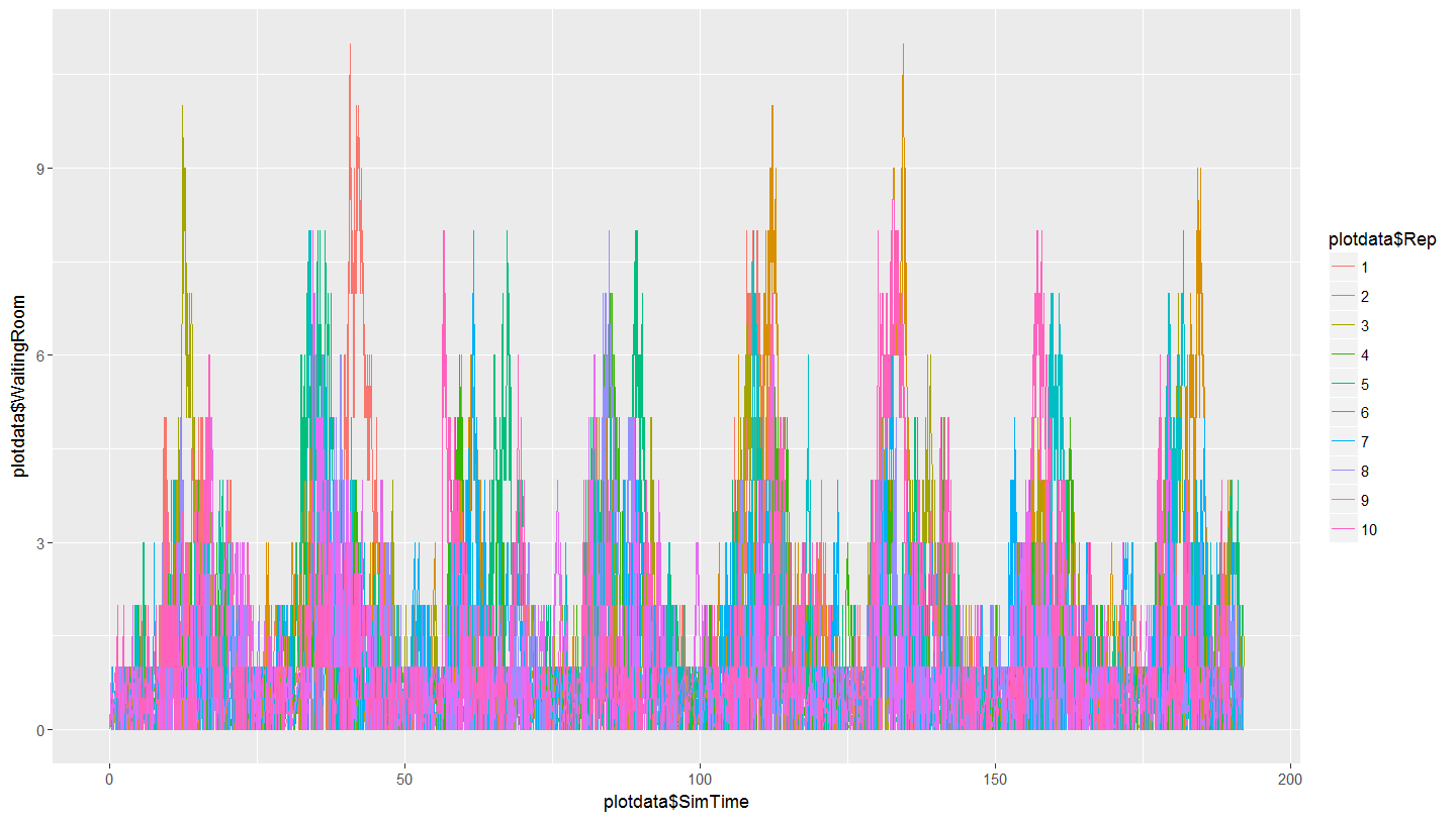 Note the cyclical nature of the plot that demonstrates the daily effect of the variable arrival rates for walk-up patients.
Return to top
Note the cyclical nature of the plot that demonstrates the daily effect of the variable arrival rates for walk-up patients.
Return to top
Conclusions
In this case study, you extended the SHC with Scheduled Appointments models to a triage/testing process, "noise" on appointment patient arrivals, and non-stationary arrival rates for walk-up patients. You investigated the effect of the changes as well as plotting the number in the waiting room over time to see the effect of non-stationarity. Given the imbalance between the utilisation of the doctors, how should the two doctors be rostered to ensure their workload is equitable? Return to top

| I | Attachment | History | Action | Size | Date | Who | Comment |
|---|---|---|---|---|---|---|---|
| |
Lab3Analysis.R | r4 r3 r2 r1 | manage | 1.7 K | 2017-10-01 - 22:19 | MichaelOSullivan | |
| |
nurse.png | r1 | manage | 5.1 K | 2017-09-28 - 02:44 | MichaelOSullivan | |
| |
parse_multiple_runs_log.R | r1 | manage | 2.1 K | 2017-09-29 - 02:38 | MichaelOSullivan | |
| |
parse_single_run_log.R | r1 | manage | 2.0 K | 2017-09-29 - 02:38 | MichaelOSullivan |
Topic revision: r12 - 2019-10-07 - MichaelOSullivan

Ideas, requests, problems regarding TWiki? Send feedback