Case Study: Input and Output for a Courier Service Model
Submitted: 28 Aug 2009
Operations Research Topics: SimulationModelling
Application Areas: Logistics
Contents
Problem Description
This case study is an extension of the Modelling Requests to a Courier Service case study. It examines ways to determine the inputs for the simulation model and also how to analyse the outputs from the simulation. Before starting this case study you will need to complete the Modelling Requests to a Courier Service case study. Return to topProblem Formulation
See the Modelling Requests to a Courier Service case study for the details of the problem formulation. The complete logic for the model is shown as an Arena model in Figure 1. Figure 1 Arena model for a courier service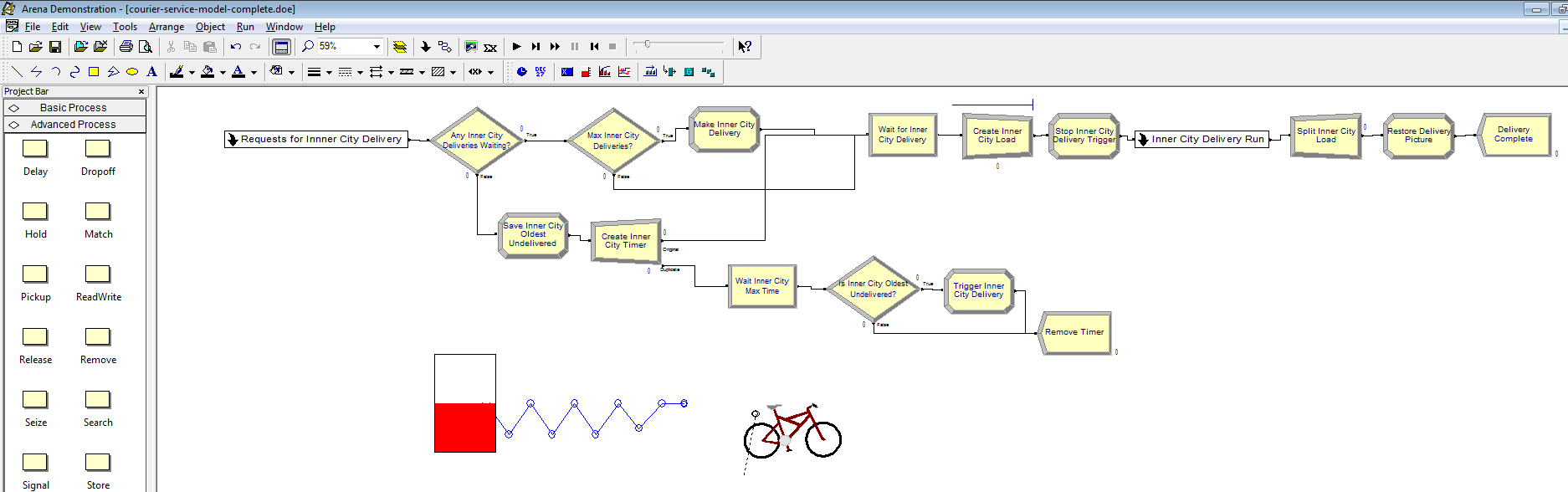 Return to top
Computational Model
Finding Input Distributions
As discussed previously, the courier company has recorded data on their delivery requests and delivery runs. This data is given courier.xls. We can use Arena's built-in Input Analyzer to determine distributions that fit the data well. First, we need to break the data up into separate text files as shown in Figure 5. Figure 5 Splitting data into text files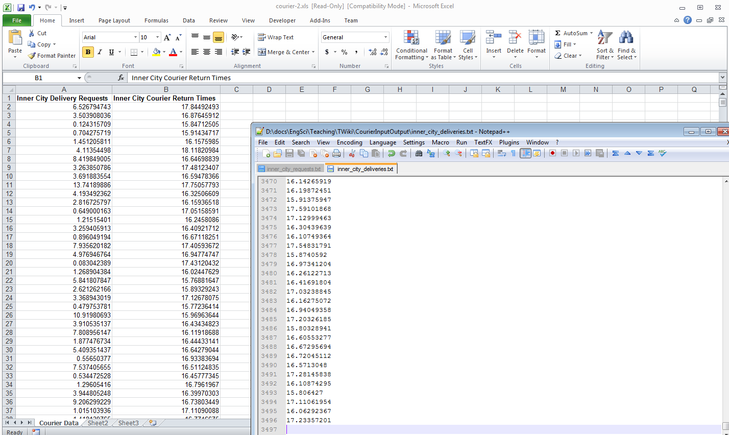 Then, we can use the Input Analyzer:
Analysing Inner City delivery requests
The Input Analyzer uses the Chi Square and Kolmogorov-Smirnov goodness-of-fit tests to determine which distributions fit best.
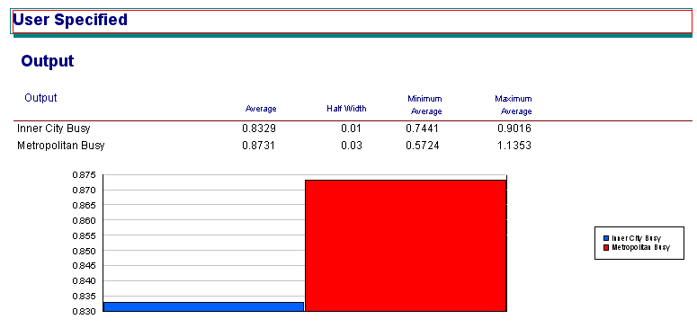
Once you have determined the best distributions, you can cut-and-paste their expressions into the appropriate submodels and run your simulation model again. Some results are shown in Figure 6.
Figure 6 Results after input analysis
Then, we can use the Input Analyzer:
Analysing Inner City delivery requests
The Input Analyzer uses the Chi Square and Kolmogorov-Smirnov goodness-of-fit tests to determine which distributions fit best.
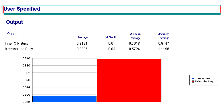
Once you have determined the best distributions, you can cut-and-paste their expressions into the appropriate submodels and run your simulation model again. Some results are shown in Figure 6.
Figure 6 Results after input analysis

Using the Data
IMPORTANT You should save your model file under a new name before adding the empirical distributions as shown below. In the Results section we will compare the 2 model files. Instead of using the Input Analyzer to estimate distributions, we can use the empirical distribution. The empirical distribution uses the histogram of the data to create a cumulative distribution function which it then uses to generate either discrete or continuous observations. In this example we will use the continuous distribution to generate interarrival times and processing times, i.e., the time taken for a courier run. Determining the Empirical Distribution Once you have changed the generation of delivery requests and the time taken to do courier runs to use empirical distributions, you can run your model again. However, you may get an error complaining about using a value of 0.00 for an interarrival time. The first entry of your empirical distributions is (0.00, 0.00, ...), i.e., there is a very small (0.00 to 3 significant figures) chance of an observation of 0.00. If this happens an infinite number of times for an interarrival time (very small probability, but theoretically possible), then there may be an infinite loop, so Arena does not allow this. Simply remove the first 2 0.00 entries (thus removing the possibility of a 0.00 interarrival time, a reasonable assumption) and your Arena model will run. Return to topResults
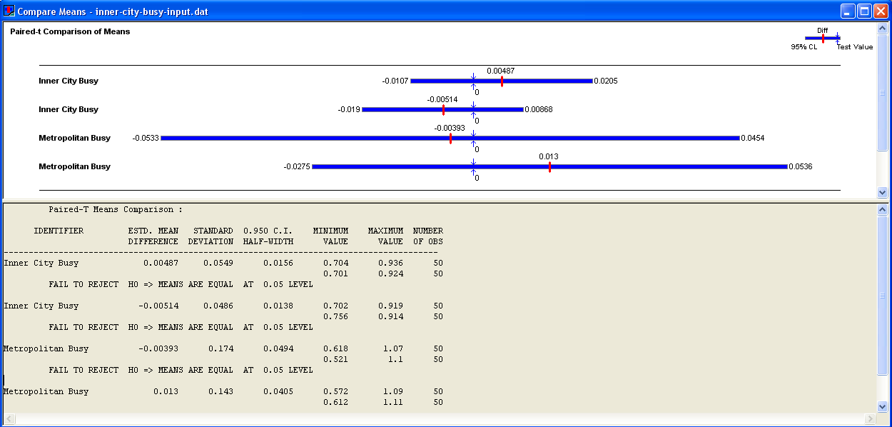
Now we have finished building simulation models with different input distributions, we will compare our models. We can compare two simulations by creating data files giving output for each replication and comparing them in Arena's Output Analyzer. First, add a Statistic to both models that records the average utilization of the Inner City Courier and the Metropolitan Courier. Adding Output Statistics to Courier Model Repeat this for your simulation model that uses the fitted distributions, but make sure to give your output files different names. Next, we can use the Output Analyzer to compare the different models. Comparing Courier Models Figure 7 shows the confidence intervals generated by Output Analyzer. They measure the difference of the mean values, i.e., average number of busy couriers, for the inner city couriers and the metropolitan couriers. The difference is the mean from the fitted distribution model (input) minus the mean from the empirical distribution model (empirical). Notice that both confidence intervals span 0, so there is no evidence of any difference between the means. We can reduce the size of the confidence intervals by reducing the variance, i.e., running more replications. Figure 7 Results after input analysis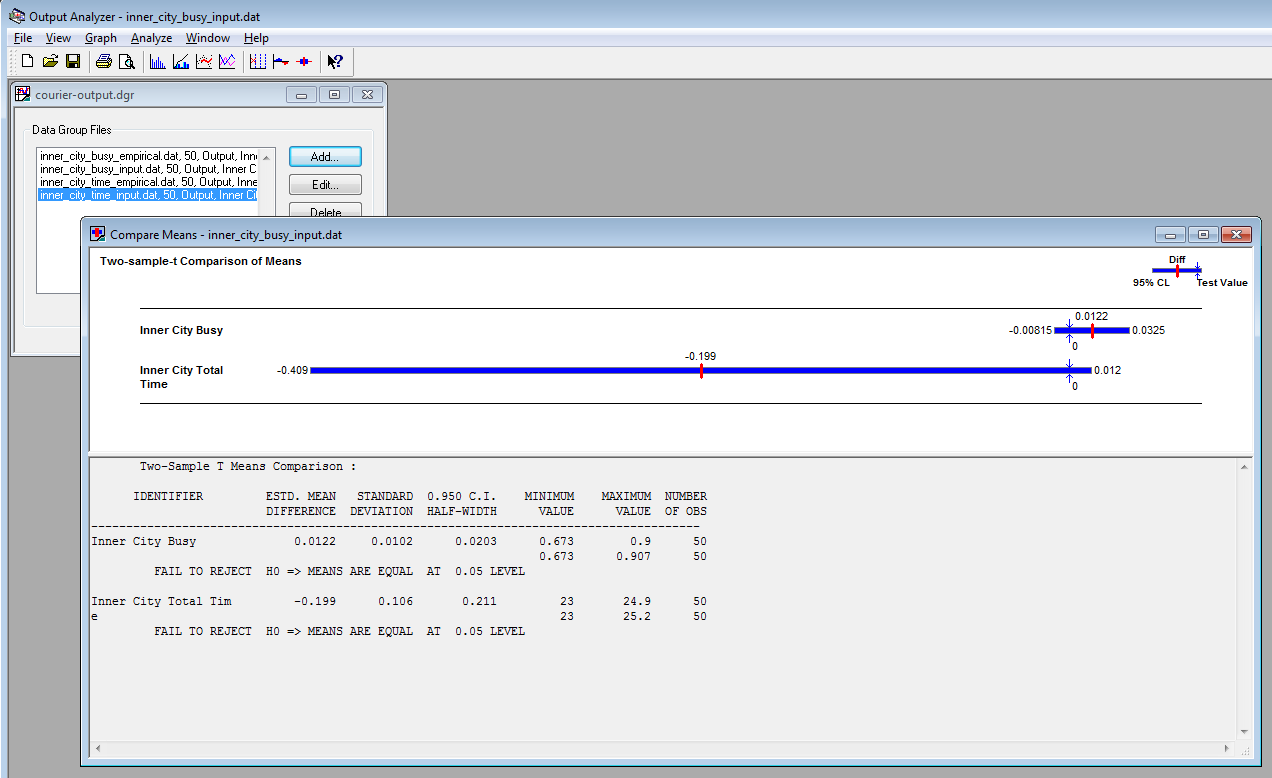 Return to top
Conclusions
The simulation model of the courier company provides different measurements of several aspects of the courier service. In this case study we looked mainly at the average number of couriers needed for both inner city and metropolitan deliveries. We considered this statistic when using a couple of different models, one that estimated distributions for the data and one that uses the empirical distribution of the data, i.e., it modelled the data explicitly. The simulation results showed that there was no evidence to reject the hypothesis that both distributions gave the same mean, i.e., average number of couriers busy, for both the inner city and metropolitan couriers. This means that we could use either approach and our results would be statistically equivalent. Return to topExtra for Experts
Arena enables you to be more selective about how random numbers are used in your simulations. This may allow you to get more accuracy in your estimates with less replications. It can also allow you to improve accuracy when comparing simulations. First, you need to add a SEEDS element to your model. Then, you add the seed to your random number expressions. The following flash movie shows how to do this and also uses the SEEDS element so that common random numbers are used across replications. Be sure to save a copy of your model before making changes. Using a SEEDS element Figure 8 shows the results for courier usage when using the empirical distribution and random numbers as usual, common random numbers and antithetic random numbers. Figure 8 Courier Usage (Empirical Distribution) with different random number utilisation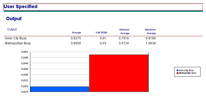
- Using random numbers as usual
- Using common random numbers
- Using antithetic random numbers
Common or Antithetic, gives a comparison with less variance. Figure 9 shows the Output Analyzer results (using a Paired-t Test because the simulations are not independent) for the previous models (without the SEEDS element - the first and third confidence intervals) and the new models (with the SEEDS element without Common or Antithetic turned on - the second and last intervals).
Figure 9 Output Analyzer Results
 However, using the
 Common option for your random numbers means that as long as you use less than 100, 000 random numbers in a single replication, each of your replications should be using exactly the same random numbers. Comparing the courier model with fitted distributions to the model with empirical distributions with both models using common random numbers in the same way gives an even greater improvement in variance. Figure 10 shows the Output Analyzer results for the previous models (without the SEEDS element - the first and third confidence intervals) and the new models (with the SEEDS element with Common turned on - the second and last intervals). Note that the confidence intervals are much smaller when using random numbers in the same way and also using Common.
Figure 10 Output Analyzer Results
 Return to top


| I | Attachment | History | Action | Size | Date | Who | Comment |
|---|---|---|---|---|---|---|---|
| |
courier-compare.swf | r1 | manage | 895.3 K | 2009-08-16 - 13:04 | MichaelOSullivan | Comparing Courier Models |
| |
courier-crn.swf | r1 | manage | 1474.1 K | 2009-08-22 - 10:22 | MichaelOSullivan | Using a SEEDS element |
| |
courier-empirical.swf | r1 | manage | 809.4 K | 2009-08-16 - 12:24 | MichaelOSullivan | Determining the Empirical Distribution |
| |
courier-input.swf | r1 | manage | 313.1 K | 2009-08-09 - 14:37 | TWikiAdminUser | Analysing Inner City delivery requests |
| |
courier-output.swf | r1 | manage | 875.9 K | 2009-08-16 - 12:50 | MichaelOSullivan | Adding Output Statistics to Courier Model |
| |
courier.xls | r1 | manage | 344.5 K | 2009-08-09 - 13:56 | TWikiAdminUser | Data from the Courier company |
This topic: OpsRes > SubmitCaseStudy > CourierServiceInputOutput
Topic revision: r7 - 2009-09-16 - MichaelOSullivan
Ideas, requests, problems regarding TWiki? Send feedback