Case Study: Calibrating the Courier Service Model

Submitted: 27 Sep 2009

Operations Research Topics: SimulationModelling

Application Areas: Logistics

Contents

• Problem Description
• Problem Formulation
• Computational Model
• Results
• Conclusions
• Extra for Experts

Problem Description

This case study extends two previous case studies:

1. Modelling Requests to a Courier Service which builds a model of a courier service receiving requests and then making deliveries;
2. Input and Output for a Courier Service Model which uses Arena tools (the Input Analyzer and Output Analyzer) to find distributions for the input to the simulation model and compares the results for fitted distributions vs empirical distributions.

In this case study we will build a simulation that uses historical data directly (instead of within an empirical distribution). Using this simulation we can estimate the total time between a request for delivery arriving at the courier service and the delivery being made.

Once we have an accurate value for the actual time a delivery request takes to be delivered, we can calibrate our fitted distributions to accurately match the real-world situation.

First, we will use Arena's Process Analyzer to simultaneously compare several different possibilities for the fitted distribution using the uniform error in the estimate of average total time (i.e., the time between a delivery request arriving and the delivery being made). Then, (in Extra for Experts, we will use Arena's OptQuest to find the best parameters for the distributions of choice by minimising the uniform error in the estimate. Finally, we will add the optimised simulation to the comparison in the Process Analyzer.

Return to top

Problem Formulation

We can easily modify the existing Courier Service Model to use the data in courier.xls because both the arrival of delivery requests and the delivery runs themselves have been abstracted into submodels.

To use the historical data to generate arrivals we simply need to step through the interarrival times for the Inner City delivery requests, wait the required time and generate the appropriate arrival.

To use the historical data to implement delivery runs we wait until a delivery run is triggered (either by the number of deliveries waiting being large enough or the time since the first undelivered request being long enough) and then use the next delivery run time from the list as the time taken for the courier to make a delivery run.

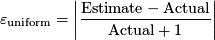
The historical data simulation gives us a "real-world" value for the average time between a delivery request arriving and the corresponding delivery being made. We can use this "actual" value to calculate the uniform error in estimates of average total time

To calibrate our simulation we need to minimise by changing the parameters to our fitted distributions. We can use black-box optimisation, in this case Tabu search via Arena's OptQuest, to determine the values of the fitted distribution parameters that provide the minimum uniform error.

Return to top

Computational Model

First, we need to name the data from each of the relevant columns of the courier.xls spreadsheet. The following flash tutorial shows how to name the Inner City data areas in an Excel 2007 spreadsheet:

Once both areas have been named: Inner_City_Deliveries; Inner_City_Return_Times; save a copy of your spreadsheet as courier-named.xls.

Now, add this file to your courier service simulation using the File data module (in the Advanced Process template). The following flash tutorial shows how add a file in Arena:

Once the file has been added we use the names defined in courier-named.xls to define Recordsets. The following flash tutorial shows how add recordsets from a file in:

Now our historical data is available for use in our simulation.

It is easiest to use the data from courier-named.xls for delivery runs first. The following flash tutorial shows how add read from a file's recordset into an attribute and then use that attribute in a Process module:

Using the historical data to generate arrivals is more complicated as we need to create entities according to the historical data. We do this by creating a logical entity in a loop. This entity is created at the start of the replication and reads the interarrival time for the next arrival. The following flash tutorial shows how create the generator logical entity and read from a file's recordset:

Once the interarrival time has been read, the generator entity delays for the interarrival time and then uses a Separate module to create a request before looping back to read the next interarrival time. The following flash tutorial shows how wait for the interarrival time, create a request entity and loop back to read more interarrival times:

Once the new entity has been created, we need to turn it into the appropriate request and send it into the rest of our model. The following flash tutorial shows how create a delivery request entity and send it to rest of the model:

Now we have a simulation that uses historical data. However, we need to see how long we can use the historical data before it repeats (Arena goes back to the start of a Recordset when it runs out of data). If we sum each of the columns in courier-names.xls and convert it from minutes into 8-hour days, we see that the Inner City Deliveries data (the time between Inner City delivery requests) provides just over 30 days of data. All the other columns provide enough data for longer durations. We set the number of replications for the historical data simulation to be 30, with each replication running for 8 hours.

Return to top

Results

Now we have a historical simulation, we can run the simulation and look at statistics from the real-world courier service. Figure 1 shows the Category Overview report with total time both Inner City deliveries, averaged over the 30 replications.

Figure 1 Total Time from the Historical Simulation

Comparing Multiple Simulations

First, we will use the Process Analyzer to compare the historical simulation with both the simulation with fitted distributions and the simulation with empirical distributions. The following flash shows how to add the three simulation models to the Process Analyzer.

IMPORTANT. You should set all the simulations (historical, fitted distributions, empirical distributions) to run in batch mode. You can do this by opening the simulation in Arena and selecting Run > Run Control > Batch Run (No Animation). To make sure the simulation's run file is properly set up for the Process Analyzer you should select Run > Check Model (or use the shortcut F4).

Next, we will insert some responses to compare amongst our simulation models. The following flash shows how insert responses and run the Process Analyzer:

After all the simulations have run in the Process Analyzer, we can use Box-and-Whisker plots to compare the confidence intervals for the total time from all the simulations simultaneously. The following flash shows how create Box-and-Whisker plots in the Process Analyzer:

The box in the Box-and-Whisker plots shows the 95% confidence interval and both the fitted and the empirical distributions give confidence intervals that overlap with the historical simulation confidence intervals for Inner City total delivery time. However, the fitted distributions don't give a confidence interval that overlaps for Metropolitan total delivery time (hence Fitted is blue while the other scenarios are red).

Changing Distribution Parameters

We can experiment with different distribution values for the fitted distributions to see if we can get a better match. The current distributions are:

In order to change these values dynamically we need to parameterise the distributions. Add the following variables to the Variable data module:

and use them to define the appropriate distributions

Now select Run > Check Model to create the simulation run file. Next, create 2 new scenarios in your Process Analyzer file, both that use your new simulation run file. The following flash shows update the Fitted scenario and add two alternatives:

Now, we want to add the distribution parameters as controls so we can experiment with them. We will see what happens when we increase and decrease the delivery time for the Metropolitan courier. We will add Metropolitan Delivery Constant as a control and set it to be 9 and 13 in the two experimental scenarios. The following flash shows how add controls to scenarios and change their values:

After running these scenarios (you may need to select Run > Reset for you original Fitted scenario) you can generate your Box-and-Whisker plot for MetropolitanDelivery.TotalTime again. You should see results like those in Figure 2.

Figure 2 Comparing scenarios in the Process Analyzer

Our experiments show that increasing the constant term in the Metropolitan Delivery distribution expression gives a better "match" for the total time to deliver Metropolitan requests.To fully explore the possibilities for the fitted distributions we can will minimise the uniform error using OptQuest (see Extra for Experts).

Return to top

Conclusions

In this case study we have used historical data and the Process Analyzer to calibrate our simulation model.

The historical data was used within our simulation model to get actual values for the total time for courier deliveries.

Once these actual values were calculated, we compared to our previous models using the Process Analyzer to experiment with different parameters for the distributions previously fitted to the historical data (in Input and Output for a Courier Service Model) to try and calibrate our model.

In Extra for Experts we use OptQuest to minimise the uniform error and automatically calibrate our fitted distributions. The calibrated fitted model is then compared to the simulation model with historical data. The calibrated model seems to provide a better fit, although further simulation work and statistical analysis is needed to confirm this.

Return to top

Extra for Experts

Minimising Uniform Error via _OptQuest

The "actual" values for the total delivery time is 23.754 minutes for an Inner City request and 52.535 for a Metropolitan request. We can add these values as Variable_s to our model and then use _OptQuest to find the best overall fit to the historical data. The following flash shows how add the actual values as Variable_s and how to start _OptQuest:

Next, we select all the parameters of the fitted distributions as well as our new InnerCityActualTotal and MetropolitanActualTotal Variable_s as controls. (We assume that we have selected the correct distributions and only need to fine tine their parameters.) The following flash shows how set the _OptQuest controls:

As responses we only need the total time for the Inner City requests and Metropolitan requests to go through the courier system. The following flash shows how set the OptQuest responses and move to the objective:

There are no constraints for this optimisation problem, so we move on to the objective (i.e., to calibrate the distribution parameters). Rather than use the absolute value for the uniform error, we calculate the squared uniform error for both Inner City deliveries and Metropolitan deliveries and use the sum of these values. This squared sum will hopefully provide the Tabu search with better impetus to find the minimum uniform error (if the solution is far from the minimum error, the squared error will be much greater than the absolute error). The following flash shows how set the OptQuest objective:

The objective is minimised by changing the controls within the ranges specified (we accepted the defaults when we set the controls). However, we don't want InnerCityActualTotal and MetropolitanActualTotal to change, so we must fix their ranges. The following flash shows how adjust possible ranges of values for controls in OptQuest:

Now, we are all set to run our optimisation. We set some options to allow for the number of replication to vary between 10 and 50 until the 95% confidence interval is within 10% of the mean and then run OptQuest. The following flash shows how set options and start OptQuest solving:

After 179 simulation runs in OptQuest, the best values for the parameters (from simulation run 60) can be seen in Figure 3.

Figure 3 Automatic calibration using OptQuest

Using these parameters and checking the Box-and-Whisker plot from the Process Analyzer shows that the best solution after 179 simulations is a reasonable match to the historical simulation (see Figure 4).

Figure 4 Comparing OptQuest solution using Process Analyzer

Return to top