
Difference: SupplyChainMP (1 vs. 15)
Revision 152018-11-23 - TWikiAdminUser
| Line: 1 to 1 | |||||||||||||||||||||||||||||||||||||||||||||||||||||||||||||||
|---|---|---|---|---|---|---|---|---|---|---|---|---|---|---|---|---|---|---|---|---|---|---|---|---|---|---|---|---|---|---|---|---|---|---|---|---|---|---|---|---|---|---|---|---|---|---|---|---|---|---|---|---|---|---|---|---|---|---|---|---|---|---|---|
<-- Ready to Review --> | |||||||||||||||||||||||||||||||||||||||||||||||||||||||||||||||
| Line: 96 to 96 | |||||||||||||||||||||||||||||||||||||||||||||||||||||||||||||||
-- MichaelOSullivan - 31 Mar 2008
| |||||||||||||||||||||||||||||||||||||||||||||||||||||||||||||||
| Changed: | |||||||||||||||||||||||||||||||||||||||||||||||||||||||||||||||
| < < |
| ||||||||||||||||||||||||||||||||||||||||||||||||||||||||||||||
| > > |
| ||||||||||||||||||||||||||||||||||||||||||||||||||||||||||||||
Revision 142009-10-06 - MichaelOSullivan
| Line: 1 to 1 | |||||||||
|---|---|---|---|---|---|---|---|---|---|
<-- Ready to Review --> | |||||||||
| Changed: | |||||||||
| < < | %BEGINLATEXPREAMBLE% \usepackage{amsmath} \usepackage{amssymb} | ||||||||
| > > | %BEGINLATEXPREAMBLE% \usepackage{amsmath} \usepackage{amssymb} | ||||||||
%ENDLATEXPREAMBLE%
Supply Chain Mathematical Programmes | |||||||||
| Line: 21 to 19 | |||||||||
Introduction | |||||||||
| Changed: | |||||||||
| < < | Throughout a supply chain there are many organisations who are trying to make the best decision for their business. These decisions can be formulated as mathematical programmes. We will introduce a supply chain model that is a simplification of that presented in the Supply Chains introduction. We will formulate the mathematical programmes faced by the organisations at each stage of this supply chain. This simplification can be easily extended to supply chain models with more stages (e.g., see Supply Chains) by inserting more Retailer's Problems into the simplfied model. | ||||||||
| > > | Throughout a supply chain there are many organisations who are trying to make the best decision for their business. These decisions can be formulated as mathematical programmes. We will introduce a supply chain model that is a simplification of that presented in the Supply Chains introduction. We will formulate the mathematical programmes faced by the organisations at each stage of this supply chain. This simplification can be easily extended to supply chain models with more stages (e.g., see Supply Chains) by inserting more Retailer's Problems into the simplified model. | ||||||||
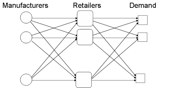
The supply chain model considered here has three stages (shown in Figure 1):
| |||||||||
| Changed: | |||||||||
| < < |
| ||||||||
| > > |
| ||||||||
Figure 1 A 3-stage supply chain model (adapted from Supply Chain Network Economics ) | |||||||||
| Changed: | |||||||||
| < < |  | ||||||||
| > > | | ||||||||
| The rest of this topic deals with the mathematical programmes faced by the manufacturers, retailers and consumers (in the demand markets). | |||||||||
| Line: 39 to 36 | |||||||||
The Manufacturer's Problem | |||||||||
| Changed: | |||||||||
| < < | Each manufacturer  (from the set of manufacturers  must determine an optimal output quantity  which is split into flows  to send to each retailer  (from the set of retailers  ). Of course all output is sent to retailers so  | ||||||||
| > > | Each manufacturer (from the set of manufacturers must determine an optimal output quantity which is split into flows to send to each retailer (from the set of retailers ). Of course all output is sent to retailers so | ||||||||
| Changed: | |||||||||
| < < | The production cost  for manufacturer may be influenced not only by their output , but also by the outputs from other manufacturers, e.g., due the competition for shared resources. Thus, is a function of the vector  which may also be expressed as the matrix of flows from manufacturers to retailers, i.e.,    associated with sending flow from manufacturer to retailer , i.e.,  sets a unit price  for selling their output to retailer . Now manufacturer want to maximise their profit, i.e., total income - production cost - transaction cost, over the set of nonegative flows:
%BEGINLATEX{label="eq:manufacturer"}%
\begin{equation*}
\begin{array}{l@{ }l}
\displaystyle \max \sum_{j=1}^n \rho_{1ij} & \displaystyle q_{ij} - f_i(Q^1) - \sum_{j=1}^n c_{ij}(q_{ij}) \\text{subject to} \& q_{ij} \geq 0, j = 1, 2, \ldots, n
\end{array}
\end{equation*} | ||||||||
| > > | The production cost for manufacturer may be influenced not only by their output , but also by the outputs from other manufacturers, e.g., due the competition for shared resources. Thus, is a function of the vector which may also be expressed as the matrix of flows from manufacturers to retailers, i.e., associated with sending flow from manufacturer to retailer , i.e., sets a unit price for selling their output to retailer . Now manufacturer want to maximise their profit, i.e., total income - production cost - transaction cost, over the set of non-negative flows:
%BEGINLATEX{label="eq:manufacturer"}% \begin{equation*} \begin{array}{l@{ }l} \displaystyle \max \sum_{j=1}^n \rho_{1ij} & \displaystyle q_{ij} - f_i(Q^1) - \sum_{j=1}^n c_{ij}(q_{ij}) \ \text{subject to} \ & q_{ij} \geq 0, j = 1, 2, \ldots, n \end{array} \end{equation*} | ||||||||
| %ENDLATEX% Return to top | |||||||||
| Line: 67 to 52 | |||||||||
Each retailer must determine their optimal flow to receive from manufacturer and also their optimal flow  to sell to consumers in demand market  (in the set of demand markets  ). | |||||||||
| Changed: | |||||||||
| < < | There is an associated handling cost  that may depend on the flow to other retailers, e.g., competition for output from the manufacturers:  | ||||||||
| > > | There is an associated handling cost that may depend on the flow to other retailers, e.g., competition for output from the manufacturers: | ||||||||
Each retailer sets a unit price  for sending flow to a demand market. Note that this price does not depend on the market (as consumers will simply move to the demand markets with the lowest price).
Now the retailer must choose flows to maximise their total profit (total income - handling cost - purchase cost): | |||||||||
| Changed: | |||||||||
| < < | %BEGINLATEX{label="eq:retailer"}% \begin{equation*} \begin{array}{l@{ }l@{ }l} \displaystyle \max \rho_{2j} \sum_{k=1}^p & q_{jk} & \displaystyle - \ c_j(Q^1) - \sum_{i=1}^m \rho_{1ij} q_{ij} \\text{subject to} \\displaystyle \hfill \sum_{k=1}^p & q_{jk} & \displaystyle \leq \sum_{i=1}^m q_{ij} \& q_{ij} &\geq 0, i = 1, 2, \ldots, m \& q_{jk} &\geq 0, k = 1, 2, \ldots, p \end{array} \end{equation*} | ||||||||
| > > | %BEGINLATEX{label="eq:retailer"}% \begin{equation*} \begin{array}{l@{ }l@{ }l} \displaystyle \max \rho_{2j} \sum_{k=1}^p & q_{jk} & \displaystyle - \ c_j(Q^1) - \sum_{i=1}^m \rho_{1ij} q_{ij} \ \text{subject to} \ \displaystyle \hfill \sum_{k=1}^p & q_{jk} & \displaystyle \leq \sum_{i=1}^m q_{ij} \ & q_{ij} &\geq 0, i = 1, 2, \ldots, m \ & q_{jk} &\geq 0, k = 1, 2, \ldots, p \end{array} \end{equation*} | ||||||||
%ENDLATEX%
Return to top
The Consumers' Problem | |||||||||
| Changed: | |||||||||
| < < | The consumers within a demand market must determine how much of the incoming flow to purchase. They take the price from each retailer and there is an associated unit transaction cost  for purchasing flow from retailer . This cost may depend on the behaviour of consumers in other demand markets, e.g., . competition for flows from retailers, i.e.,   | ||||||||
| > > | The consumers within a demand market must determine how much of the incoming flow to purchase. They take the price from each retailer and there is an associated unit transaction cost for purchasing flow from retailer . This cost may depend on the behaviour of consumers in other demand markets, e.g., . competition for flows from retailers, i.e., | ||||||||
The combination of the different prices and unit transaction costs gives rise to an "effective" price  for a consumer to purchase a unit of flow in demand market . | |||||||||
| Changed: | |||||||||
| < < | The demand for flow in demand market is determined by the demand curve, a function of the effective price, i.e.,
 | ||||||||
| > > | The demand for flow in demand market is determined by the demand curve, a function of the effective price, i.e., | ||||||||
|
The consumers within demand market choose flows to minimise their total cost while meeting demand: | |||||||||
| Changed: | |||||||||
| < < | %BEGINLATEX{label="eq:consumer"}% \begin{equation*} \begin{array}{l@{ }l@{ }l} \displaystyle \min \rho_{3k} \sum_{j=1}^n & q_{jk} \\text{subject to} \\displaystyle \hfill \sum_{j=1}^n & q_{jk} & \geq d_k(\rho_{3k}) \& q_{jk} &\geq 0, j = 1, 2, \ldots, n \end{array} \end{equation*} | ||||||||
| > > | %BEGINLATEX{label="eq:consumer"}% \begin{equation*} \begin{array}{l@{ }l@{ }l} \displaystyle \min \rho_{3k} \sum_{j=1}^n & q_{jk} \ \text{subject to} \ \displaystyle \hfill \sum_{j=1}^n & q_{jk} & \geq d_k(\rho_{3k}) \ & q_{jk} &\geq 0, j = 1, 2, \ldots, n \end{array} \end{equation*} | ||||||||
%ENDLATEX%
Return to top
Equilibrium and Variational Inequalities | |||||||||
| Changed: | |||||||||
| < < | If the prices , and  are not coordinated then solving the Manufacturer's Problem, the Retailer's Problem and the Consumers' Problem will give inconsistent values for and . That is, the manufacturers will want to ship different ammounts to the retailers than the retailers will want to receive from the maunfacturers and the retailers will want to sell different amounts to the demand markets from the amounts that the consumers at the demand markets want to purchase. However, these prices will adjust until the supply chain reaches equilibrium and the flows from the different mathematical programmes agree. | ||||||||
| > > | If the prices , and are not coordinated then solving the Manufacturer's Problem, the Retailer's Problem and the Consumers' Problem will give inconsistent values for and . That is, the manufacturers will want to ship different amounts to the retailers than the retailers will want to receive from the manufacturers and the retailers will want to sell different amounts to the demand markets from the amounts that the consumers at the demand markets want to purchase. However, these prices will adjust until the supply chain reaches equilibrium and the flows from the different mathematical programmes agree. | ||||||||
One way to find this equilibrium point is to solve a variational inequality. Theorem 1 gives the necessary variational inequalities:
Theorem 1: Variational Inequality The equilibrium state governing the supply chain model according to the optimality conditions of the supply chain mathematical programmes (?? REFLATEX{eq:manufacturer} not defined in eqn list ??), (?? REFLATEX{eq:retailer} not defined in eqn list ??) and (?? REFLATEX{eq:consumer} not defined in eqn list ??) is equivalent to the solution of the variational inequality problem given by: determine the equilibrium vectors of product shipments, shadow prices, and demand market prices  satisfying | |||||||||
| Changed: | |||||||||
| < < | %BEGINLATEX% \begin{equation*} \begin{split} & \sum_{i=1}^m \sum_{j=1}^n \left[ \frac{\partial f_i(Q^{1*})}{\partial q_{ij}} + \frac{\partial c_{ij}(q_{ij}^*)}{\partial q_{ij}} + \frac{\partial c_j(Q^{1*})}{\partial q_{ij}} - \gamma_j^* \right] \times \left[ q_{ij} - q_{ij}^* \right] \&+ \sum_{j=1}^n \sum_{k=1}^p \left[ c_{jk}(Q^{2*}) + \gamma_j^* - \rho_{3k}^* \right] \times \left[ q_{jk} - q_{jk}^* \right] \&+ \sum_{j=1}^n \left[ \sum_{i=1}^m q_{ij}^* - \sum_{k=1}^p q_{jk}^* \right] \times \left[ \gamma_j - \gamma_j^* \right] \&+ \sum_{k=1}^p \left[ \sum_{j=1}^n q_{jk}^* - d_k(\rho_3^*) \right] \times \left[ \rho_{3k} - \rho_{3k}^* \right] \geq 0, \forall (Q^{1}, Q^{2}, \gamma, \rho_{3}) \in \mathbb{R}_+^{mn+np+n+p} \end{split} \end{equation*} | ||||||||
| > > | %BEGINLATEX% \begin{equation*} \begin{split} & \sum_{i=1}^m \sum_{j=1}^n \left[ \frac{\partial f_i(Q^{1*})}{\partial q_{ij}} + \frac{\partial c_{ij}(q_{ij}^*)}{\partial q_{ij}} + \frac{\partial c_j(Q^{1*})}{\partial q_{ij}} - \gamma_j^* \right] \times \left[ q_{ij} - q_{ij}^* \right] \ &+ \sum_{j=1}^n \sum_{k=1}^p \left[ c_{jk}(Q^{2*}) + \gamma_j^* - \rho_{3k}^* \right] \times \left[ q_{jk} - q_{jk}^* \right] \ &+ \sum_{j=1}^n \left[ \sum_{i=1}^m q_{ij}^* - \sum_{k=1}^p q_{jk}^* \right] \times \left[ \gamma_j - \gamma_j^* \right] \ &+ \sum_{k=1}^p \left[ \sum_{j=1}^n q_{jk}^* - d_k(\rho_3^*) \right] \times \left[ \rho_{3k} - \rho_{3k}^* \right] \geq 0, \forall (Q^{1}, Q^{2}, \gamma, \rho_{3}) \in \mathbb{R}_+^{mn+np+n+p} \end{split} \end{equation*} | ||||||||
| %ENDLATEX% Once the equilibrium state has been found the manufacturers' prices and the retailers' prices can be calculated: | |||||||||
| Line: 168 to 123 | |||||||||
| |||||||||
| Deleted: | |||||||||
| < < |
| ||||||||
| |||||||||
Revision 132008-04-20 - TWikiAdminUser
| Line: 1 to 1 | ||||||||
|---|---|---|---|---|---|---|---|---|
<-- Ready to Review --> | ||||||||
| Line: 117 to 117 | ||||||||
|
If the prices , and are not coordinated then solving the Manufacturer's Problem, the Retailer's Problem and the Consumers' Problem will give inconsistent values for and . That is, the manufacturers will want to ship different ammounts to the retailers than the retailers will want to receive from the maunfacturers and the retailers will want to sell different amounts to the demand markets from the amounts that the consumers at the demand markets want to purchase. However, these prices will adjust until the supply chain reaches equilibrium and the flows from the different mathematical programmes agree. | ||||||||
| Changed: | ||||||||
| < < | One way to find this equilibrium point is to solve a [[https://en.wikipedia.org/wiki/Variational_inequality][variational inequality]. Theorem 1 gives the necessary variational inequalities: | |||||||
| > > | One way to find this equilibrium point is to solve a variational inequality. Theorem 1 gives the necessary variational inequalities: | |||||||
|
Theorem 1: Variational Inequality The equilibrium state governing the supply chain model according to the optimality conditions of the supply chain mathematical programmes (?? REFLATEX{eq:manufacturer} not defined in eqn list ??), (?? REFLATEX{eq:retailer} not defined in eqn list ??) and (?? REFLATEX{eq:consumer} not defined in eqn list ??) is equivalent to the solution of the variational inequality problem given by: determine the equilibrium vectors of product shipments, shadow prices, and demand market prices satisfying | ||||||||
Revision 122008-04-01 - MichaelOSullivan
| Line: 1 to 1 | |||||||||
|---|---|---|---|---|---|---|---|---|---|
| |||||||||
| Added: | |||||||||
| > > | <-- Ready to Review --> | ||||||||
| %BEGINLATEXPREAMBLE% \usepackage{amsmath} \usepackage{amssymb} | |||||||||
| Line: 115 to 117 | |||||||||
|
If the prices , and are not coordinated then solving the Manufacturer's Problem, the Retailer's Problem and the Consumers' Problem will give inconsistent values for and . That is, the manufacturers will want to ship different ammounts to the retailers than the retailers will want to receive from the maunfacturers and the retailers will want to sell different amounts to the demand markets from the amounts that the consumers at the demand markets want to purchase. However, these prices will adjust until the supply chain reaches equilibrium and the flows from the different mathematical programmes agree. | |||||||||
| Changed: | |||||||||
| < < | One way to find this equilibrium point is to solve a [[VariationalInequalities][variational inequality]. Theorem 1 gives the necessary variational inequalities: | ||||||||
| > > | One way to find this equilibrium point is to solve a [[https://en.wikipedia.org/wiki/Variational_inequality][variational inequality]. Theorem 1 gives the necessary variational inequalities: | ||||||||
|
Theorem 1: Variational Inequality The equilibrium state governing the supply chain model according to the optimality conditions of the supply chain mathematical programmes (?? REFLATEX{eq:manufacturer} not defined in eqn list ??), (?? REFLATEX{eq:retailer} not defined in eqn list ??) and (?? REFLATEX{eq:consumer} not defined in eqn list ??) is equivalent to the solution of the variational inequality problem given by: determine the equilibrium vectors of product shipments, shadow prices, and demand market prices satisfying | |||||||||
| Added: | |||||||||
| > > | |||||||||
| %BEGINLATEX% \begin{equation*} \begin{split} | |||||||||
| Line: 129 to 132 | |||||||||
| \end{equation*} %ENDLATEX% | |||||||||
| Added: | |||||||||
| > > | Once the equilibrium state has been found the manufacturers' prices and the retailers' prices can be calculated:
| ||||||||
| Return to top -- MichaelOSullivan - 31 Mar 2008 | |||||||||
| Line: 165 to 172 | |||||||||
| |||||||||
| Added: | |||||||||
| > > |
| ||||||||
 if
 ;
 if
 for some
Revision 112008-04-01 - MichaelOSullivan
| Line: 1 to 1 | ||||||||
|---|---|---|---|---|---|---|---|---|
| ||||||||
| Line: 124 to 124 | ||||||||
| & \sum_{i=1}^m \sum_{j=1}^n \left[ \frac{\partial f_i(Q^{1*})}{\partial q_{ij}} + \frac{\partial c_{ij}(q_{ij}^*)}{\partial q_{ij}} + \frac{\partial c_j(Q^{1*})}{\partial q_{ij}} - \gamma_j^* \right] \times \left[ q_{ij} - q_{ij}^* \right] \&+ \sum_{j=1}^n \sum_{k=1}^p \left[ c_{jk}(Q^{2*}) + \gamma_j^* - \rho_{3k}^* \right] \times \left[ q_{jk} - q_{jk}^* \right] \&+ \sum_{j=1}^n \left[ \sum_{i=1}^m q_{ij}^* - \sum_{k=1}^p q_{jk}^* \right] \times \left[ \gamma_j - \gamma_j^* \right] \ | ||||||||
| Changed: | ||||||||
| < < | &+ \sum | |||||||
| > > | &+ \sum_{k=1}^p \left[ \sum_{j=1}^n q_{jk}^* - d_k(\rho_3^*) \right] \times \left[ \rho_{3k} - \rho_{3k}^* \right] \geq 0, \forall (Q^{1}, Q^{2}, \gamma, \rho_{3}) \in \mathbb{R}_+^{mn+np+n+p} | |||||||
| \end{split} \end{equation*} %ENDLATEX% | ||||||||
| Line: 164 to 164 | ||||||||
| ||||||||
| Changed: | ||||||||
| < < |
| |||||||
| > > |
| |||||||
Revision 102008-04-01 - MichaelOSullivan
| Line: 1 to 1 | |||||||||
|---|---|---|---|---|---|---|---|---|---|
| |||||||||
| Line: 49 to 49 | |||||||||
| sets a unit price for selling their output to retailer . Now manufacturer want to maximise their profit, i.e., total income - production cost - transaction cost, over the set of nonegative flows: | |||||||||
| Changed: | |||||||||
| < < | %BEGINLATEX{label="eq:manufacturer}% | ||||||||
| > > | %BEGINLATEX{label="eq:manufacturer"}% | ||||||||
| \begin{equation*} \begin{array}{l@{ }l} \displaystyle \max \sum_{j=1}^n \rho_{1ij} & \displaystyle q_{ij} - f_i(Q^1) - \sum_{j=1}^n c_{ij}(q_{ij}) \ | |||||||||
| Line: 71 to 71 | |||||||||
| Each retailer sets a unit price for sending flow to a demand market. Note that this price does not depend on the market (as consumers will simply move to the demand markets with the lowest price).
Now the retailer must choose flows to maximise their total profit (total income - handling cost - purchase cost): | |||||||||
| Changed: | |||||||||
| < < | %BEGINLATEX{label="eq:retailer}% | ||||||||
| > > | %BEGINLATEX{label="eq:retailer"}% | ||||||||
| \begin{equation*} \begin{array}{l@{ }l@{ }l} \displaystyle \max \rho_{2j} \sum_{k=1}^p & q_{jk} & \displaystyle - \ c_j(Q^1) - \sum_{i=1}^m \rho_{1ij} q_{ij} \ | |||||||||
| Line: 98 to 98 | |||||||||
| choose flows to minimise their total cost while meeting demand: | |||||||||
| Changed: | |||||||||
| < < | %BEGINLATEX{label="eq:consumer}% | ||||||||
| > > | %BEGINLATEX{label="eq:consumer"}% | ||||||||
| \begin{equation*} \begin{array}{l@{ }l@{ }l} \displaystyle \min \rho_{3k} \sum_{j=1}^n & q_{jk} \ | |||||||||
| Line: 121 to 121 | |||||||||
| %BEGINLATEX% \begin{equation*} \begin{split} | |||||||||
| Changed: | |||||||||
| < < | & \sum_{i=1}^m \sum_{j=1}^n \left[ \frac{\partial f_i(Q^{1*})}{\partial q_{ij}} \right] \&+ \sum_{j=1}^n \sum_{k=1}^p | ||||||||
| > > | & \sum_{i=1}^m \sum_{j=1}^n \left[ \frac{\partial f_i(Q^{1*})}{\partial q_{ij}} + \frac{\partial c_{ij}(q_{ij}^*)}{\partial q_{ij}} + \frac{\partial c_j(Q^{1*})}{\partial q_{ij}} - \gamma_j^* \right] \times \left[ q_{ij} - q_{ij}^* \right] \&+ \sum_{j=1}^n \sum_{k=1}^p \left[ c_{jk}(Q^{2*}) + \gamma_j^* - \rho_{3k}^* \right] \times \left[ q_{jk} - q_{jk}^* \right] \&+ \sum_{j=1}^n \left[ \sum_{i=1}^m q_{ij}^* - \sum_{k=1}^p q_{jk}^* \right] \times \left[ \gamma_j - \gamma_j^* \right] \&+ \sum | ||||||||
| \end{split} \end{equation*} %ENDLATEX% | |||||||||
| Line: 159 to 161 | |||||||||
| |||||||||
| Changed: | |||||||||
| < < |
| ||||||||
| > > |
| ||||||||
Revision 92008-04-01 - MichaelOSullivan
| Line: 1 to 1 | |||||||||||||
|---|---|---|---|---|---|---|---|---|---|---|---|---|---|
| |||||||||||||
| Line: 49 to 49 | |||||||||||||
| sets a unit price for selling their output to retailer . Now manufacturer want to maximise their profit, i.e., total income - production cost - transaction cost, over the set of nonegative flows: | |||||||||||||
| Changed: | |||||||||||||
| < < | %BEGINLATEX% | ||||||||||||
| > > | %BEGINLATEX{label="eq:manufacturer}% | ||||||||||||
| \begin{equation*} \begin{array}{l@{ }l} \displaystyle \max \sum_{j=1}^n \rho_{1ij} & \displaystyle q_{ij} - f_i(Q^1) - \sum_{j=1}^n c_{ij}(q_{ij}) \ | |||||||||||||
| Line: 71 to 71 | |||||||||||||
| Each retailer sets a unit price for sending flow to a demand market. Note that this price does not depend on the market (as consumers will simply move to the demand markets with the lowest price).
Now the retailer must choose flows to maximise their total profit (total income - handling cost - purchase cost): | |||||||||||||
| Changed: | |||||||||||||
| < < | %BEGINLATEX% | ||||||||||||
| > > | %BEGINLATEX{label="eq:retailer}% | ||||||||||||
| \begin{equation*} \begin{array}{l@{ }l@{ }l} \displaystyle \max \rho_{2j} \sum_{k=1}^p & q_{jk} & \displaystyle - \ c_j(Q^1) - \sum_{i=1}^m \rho_{1ij} q_{ij} \ | |||||||||||||
| Line: 98 to 98 | |||||||||||||
| choose flows to minimise their total cost while meeting demand: | |||||||||||||
| Changed: | |||||||||||||
| < < | %BEGINLATEX% | ||||||||||||
| > > | %BEGINLATEX{label="eq:consumer}% | ||||||||||||
| \begin{equation*} \begin{array}{l@{ }l@{ }l} \displaystyle \min \rho_{3k} \sum_{j=1}^n & q_{jk} \ | |||||||||||||
| Line: 117 to 117 | |||||||||||||
| One way to find this equilibrium point is to solve a [[VariationalInequalities][variational inequality]. Theorem 1 gives the necessary variational inequalities: | |||||||||||||
| Changed: | |||||||||||||
| < < | *Theorem 1: Variational Inequality* _The equilibrium state governing the supply chain model according to the optimality conditions of the corresponding mathematical programmes is equivalent to the solution of the variational inequality problem given by: determine the equilibrium vectors of product shipments, shadow prices, and demand market prices satisfying | ||||||||||||
| > > | Theorem 1: Variational Inequality The equilibrium state governing the supply chain model according to the optimality conditions of the supply chain mathematical programmes (?? REFLATEX{eq:manufacturer} not defined in eqn list ??), (?? REFLATEX{eq:retailer} not defined in eqn list ??) and (?? REFLATEX{eq:consumer} not defined in eqn list ??) is equivalent to the solution of the variational inequality problem given by: determine the equilibrium vectors of product shipments, shadow prices, and demand market prices satisfying
 Latex rendering error!! dvi file was not created. | ||||||||||||
| Return to top | |||||||||||||
| Line: 138 to 146 | |||||||||||||
| |||||||||||||
| Deleted: | |||||||||||||
| < < |
| ||||||||||||
| |||||||||||||
| Deleted: | |||||||||||||
| < < |
| ||||||||||||
| |||||||||||||
| Deleted: | |||||||||||||
| < < |
| ||||||||||||
| |||||||||||||
| Added: | |||||||||||||
| > > |
| ||||||||||||
Revision 82008-04-01 - MichaelOSullivan
| Line: 1 to 1 | ||||||||
|---|---|---|---|---|---|---|---|---|
| ||||||||
| Added: | ||||||||
| > > | \usepackage{amssymb} | |||||||
%ENDLATEXPREAMBLE%
Supply Chain Mathematical Programmes | ||||||||
| Line: 100 to 101 | ||||||||
| %BEGINLATEX% \begin{equation*} \begin{array}{l@{ }l@{ }l} | ||||||||
| Changed: | ||||||||
| < < | \displaystyle \max \rho_{2j} \sum_{k=1}^p & q_{jk} & \displaystyle - \ c_j(Q^1) - \sum_{i=1}^m \rho_{1ij} q_{ij} \ | |||||||
| > > | \displaystyle \min \rho_{3k} \sum_{j=1}^n & q_{jk} \ | |||||||
| \text{subject to} \ | ||||||||
| Changed: | ||||||||
| < < | \displaystyle \hfill \sum_{k=1}^p & q_{jk} & \displaystyle \leq \sum_{i=1}^m q_{ij} \& q_{ij} &\geq 0, i = 1, 2, \ldots, m \& q_{jk} &\geq 0, k = 1, 2, \ldots, p | |||||||
| > > | \displaystyle \hfill \sum_{j=1}^n & q_{jk} & \geq d_k(\rho_{3k}) \& q_{jk} &\geq 0, j = 1, 2, \ldots, n | |||||||
| \end{array} \end{equation*} %ENDLATEX% | ||||||||
| Line: 113 to 113 | ||||||||
Equilibrium and Variational Inequalities | ||||||||
| Added: | ||||||||
| > > | If the prices , and are not coordinated then solving the Manufacturer's Problem, the Retailer's Problem and the Consumers' Problem will give inconsistent values for and . That is, the manufacturers will want to ship different ammounts to the retailers than the retailers will want to receive from the maunfacturers and the retailers will want to sell different amounts to the demand markets from the amounts that the consumers at the demand markets want to purchase. However, these prices will adjust until the supply chain reaches equilibrium and the flows from the different mathematical programmes agree.
One way to find this equilibrium point is to solve a [[VariationalInequalities][variational inequality]. Theorem 1 gives the necessary variational inequalities:
*Theorem 1: Variational Inequality* _The equilibrium state governing the supply chain model according to the optimality conditions of the corresponding mathematical programmes is equivalent to the solution of the variational inequality problem given by: determine the equilibrium vectors of product shipments, shadow prices, and demand market prices satisfying | |||||||
| Return to top -- MichaelOSullivan - 31 Mar 2008 | ||||||||
| Line: 145 to 151 | ||||||||
| ||||||||
| Added: | ||||||||
| > > |
| |||||||
Revision 72008-04-01 - MichaelOSullivan
| Line: 1 to 1 | |||||||||||||||||||||||||
|---|---|---|---|---|---|---|---|---|---|---|---|---|---|---|---|---|---|---|---|---|---|---|---|---|---|
| |||||||||||||||||||||||||
| Line: 63 to 62 | |||||||||||||||||||||||||
The Retailer's Problem | |||||||||||||||||||||||||
| Added: | |||||||||||||||||||||||||
| > > | Each retailer must determine their optimal flow to receive from manufacturer and also their optimal flow to sell to consumers in demand market (in the set of demand markets ).
There is an associated handling cost that may depend on the flow to other retailers, e.g., competition for output from the manufacturers:
sets a unit price for sending flow to a demand market. Note that this price does not depend on the market (as consumers will simply move to the demand markets with the lowest price).
Now the retailer must choose flows to maximise their total profit (total income - handling cost - purchase cost):
 Latex rendering error!! dvi file was not created. | ||||||||||||||||||||||||
| Return to top | |||||||||||||||||||||||||
| Changed: | |||||||||||||||||||||||||
| < < | The Consumer's Problem | ||||||||||||||||||||||||
| > > | The Consumers' ProblemThe consumers within a demand market must determine how much of the incoming flow to purchase. They take the price from each retailer and there is an associated unit transaction cost for purchasing flow from retailer . This cost may depend on the behaviour of consumers in other demand markets, e.g., . competition for flows from retailers, i.e.,
for a consumer to purchase a unit of flow in demand market .
The demand for flow in demand market is determined by the demand curve, a function of the effective price, i.e.,
choose flows to minimise their total cost while meeting demand:
Latex rendering error!! dvi file was not created. | ||||||||||||||||||||||||
| Return to top | |||||||||||||||||||||||||
| Line: 90 to 132 | |||||||||||||||||||||||||
| |||||||||||||||||||||||||
| Deleted: | |||||||||||||||||||||||||
| < < |
| ||||||||||||||||||||||||
| |||||||||||||||||||||||||
| Added: | |||||||||||||||||||||||||
| > > |
| ||||||||||||||||||||||||
Revision 62008-04-01 - MichaelOSullivan
| Line: 1 to 1 | |||||||||||||||||||||||||||||||||||
|---|---|---|---|---|---|---|---|---|---|---|---|---|---|---|---|---|---|---|---|---|---|---|---|---|---|---|---|---|---|---|---|---|---|---|---|
| |||||||||||||||||||||||||||||||||||
| Added: | |||||||||||||||||||||||||||||||||||
| > > | |||||||||||||||||||||||||||||||||||
Supply Chain Mathematical ProgrammesThis material is a summary of the material on supply chain networks from Chapter 2 Supply Chain Networks in Supply Chain Network Economics: Dynamics of Prices, Flows and Profits by Anna Nagurney (2006). | |||||||||||||||||||||||||||||||||||
| Line: 17 to 21 | |||||||||||||||||||||||||||||||||||
| Throughout a supply chain there are many organisations who are trying to make the best decision for their business. These decisions can be formulated as mathematical programmes. We will introduce a supply chain model that is a simplification of that presented in the Supply Chains introduction. We will formulate the mathematical programmes faced by the organisations at each stage of this supply chain. This simplification can be easily extended to supply chain models with more stages (e.g., see Supply Chains) by inserting more Retailer's Problems into the simplfied model. The supply chain model considered here has three stages (shown in Figure 1): | |||||||||||||||||||||||||||||||||||
| Changed: | |||||||||||||||||||||||||||||||||||
| < < |
| ||||||||||||||||||||||||||||||||||
| > > |
| ||||||||||||||||||||||||||||||||||
| Products are created by the manufacturers, sold to the retailers where they are stored, distributed, etc and then sold again in the demand markets to consumers.
Figure 1 A 3-stage supply chain model (adapted from Supply Chain Network Economics) | |||||||||||||||||||||||||||||||||||
| Changed: | |||||||||||||||||||||||||||||||||||
| < < |  | ||||||||||||||||||||||||||||||||||
| > > |
The rest of this topic deals with the mathematical programmes faced by the manufacturers, retailers and consumers (in the demand markets). | ||||||||||||||||||||||||||||||||||
Return to top
The Manufacturer's Problem | |||||||||||||||||||||||||||||||||||
| Added: | |||||||||||||||||||||||||||||||||||
| > > | Each manufacturer (from the set of manufacturers must determine an optimal output quantity which is split into flows to send to each retailer (from the set of retailers ). Of course all output is sent to retailers so
for manufacturer may be influenced not only by their output , but also by the outputs from other manufacturers, e.g., due the competition for shared resources. Thus, is a function of the vector which may also be expressed as the matrix of flows from manufacturers to retailers, i.e.,
associated with sending flow from manufacturer to retailer , i.e.,
sets a unit price for selling their output to retailer . Now manufacturer want to maximise their profit, i.e., total income - production cost - transaction cost, over the set of nonegative flows:
 | ||||||||||||||||||||||||||||||||||
Return to top
The Retailer's Problem | |||||||||||||||||||||||||||||||||||
| Line: 45 to 74 | |||||||||||||||||||||||||||||||||||
| Return to top -- MichaelOSullivan - 31 Mar 2008 | |||||||||||||||||||||||||||||||||||
| Deleted: | |||||||||||||||||||||||||||||||||||
| < < |
| ||||||||||||||||||||||||||||||||||
| Changed: | |||||||||||||||||||||||||||||||||||
| < < |
| ||||||||||||||||||||||||||||||||||
| > > |
| ||||||||||||||||||||||||||||||||||
Revision 52008-04-01 - MichaelOSullivan
| Line: 1 to 1 | ||||||||
|---|---|---|---|---|---|---|---|---|
Supply Chain Mathematical Programmes | ||||||||
| Changed: | ||||||||
| < < | This material is a summary of the material on supply chain networks from Chapter 2 Supply Chain Networks in Supply Chain Network Economics: Dynamics of Prices, Flows and Profits by Anna Nagurney (2006). | |||||||
| > > | This material is a summary of the material on supply chain networks from Chapter 2 Supply Chain Networks in Supply Chain Network Economics: Dynamics of Prices, Flows and Profits by Anna Nagurney (2006). | |||||||
Supply Chains | ||||||||
| Line: 14 to 14 | ||||||||
Introduction | ||||||||
| Changed: | ||||||||
| < < | Throughout a supply chain there are many organisations who are trying to make the best decision for their business. These decisions can be formulated as mathematical programmes. We will introduce a simplified version of a supply chain (cf. ) here and formulate the mathematical programmes faced by the organisations at each stage of this supply chain. | |||||||
| > > | Throughout a supply chain there are many organisations who are trying to make the best decision for their business. These decisions can be formulated as mathematical programmes. We will introduce a supply chain model that is a simplification of that presented in the Supply Chains introduction. We will formulate the mathematical programmes faced by the organisations at each stage of this supply chain. This simplification can be easily extended to supply chain models with more stages (e.g., see Supply Chains) by inserting more Retailer's Problems into the simplfied model.
The supply chain model considered here has three stages (shown in Figure 1):
)
| |||||||
| Return to top | ||||||||
| Line: 35 to 45 | ||||||||
| Return to top -- MichaelOSullivan - 31 Mar 2008 \ No newline at end of file | ||||||||
| Added: | ||||||||
| > > |
| |||||||
Revision 42008-04-01 - MichaelOSullivan
| Line: 1 to 1 | ||||||||
|---|---|---|---|---|---|---|---|---|
Supply Chain Mathematical Programmes | ||||||||
| Line: 14 to 14 | ||||||||
Introduction | ||||||||
| Changed: | ||||||||
| < < | Throughout a supply chain | |||||||
| > > | Throughout a supply chain there are many organisations who are trying to make the best decision for their business. These decisions can be formulated as mathematical programmes. We will introduce a simplified version of a supply chain (cf. ) here and formulate the mathematical programmes faced by the organisations at each stage of this supply chain. | |||||||
Return to top
The Manufacturer's Problem | ||||||||
Revision 32008-04-01 - MichaelOSullivan
| Line: 1 to 1 | ||||||||
|---|---|---|---|---|---|---|---|---|
Supply Chain Mathematical Programmes | ||||||||
| Line: 14 to 14 | ||||||||
Introduction | ||||||||
| Added: | ||||||||
| > > | Throughout a supply chain | |||||||
Return to top
The Manufacturer's Problem | ||||||||
Revision 22008-03-31 - MichaelOSullivan
| Line: 1 to 1 | ||||||||
|---|---|---|---|---|---|---|---|---|
Supply Chain Mathematical ProgrammesThis material is a summary of the material on supply chain networks from Chapter 2 Supply Chain Networks in Supply Chain Network Economics: Dynamics of Prices, Flows and Profits by Anna Nagurney (2006). | ||||||||
| Added: | ||||||||
| > > | Supply Chains
IntroductionReturn to topThe Manufacturer's ProblemReturn to topThe Retailer's ProblemReturn to topThe Consumer's ProblemReturn to topEquilibrium and Variational InequalitiesReturn to top | |||||||
| -- MichaelOSullivan - 31 Mar 2008 | ||||||||
Revision 12008-03-31 - MichaelOSullivan
| Line: 1 to 1 | ||||||||
|---|---|---|---|---|---|---|---|---|
| Added: | ||||||||
| > > |
Supply Chain Mathematical ProgrammesThis material is a summary of the material on supply chain networks from Chapter 2 Supply Chain Networks in Supply Chain Network Economics: Dynamics of Prices, Flows and Profits by Anna Nagurney (2006). -- MichaelOSullivan - 31 Mar 2008 | |||||||
View topic | History: r15 < r14 < r13 < r12 | More topic actions...

 Copyright © 2008-2026 by the contributing authors. All material on this collaboration platform is the property of the contributing authors.
Ideas, requests, problems regarding TWiki? Send feedback